Preface
Welcome to ProFacet!
ProFacet works a bit differently than other tools. Under the hood, every design is defined by a text-based "recipe" called FSL (Facet Specification Language).
You don't have to write this code yourself. As you work with the visual tools like the Interactive Slicer, ProFacet writes the FSL for you automatically. You can create entire designs just by clicking and dragging.
However, this recipe is always there, visible and editable. This means you have the best of both worlds: the ease of a visual interface and the precision of a text definition. You can switch between them at any time. While you can operate the tool entirely through the UI, most users find that they naturally start using both: the UI for the heavy lifting and the code for quick tweaks or precise adjustments.
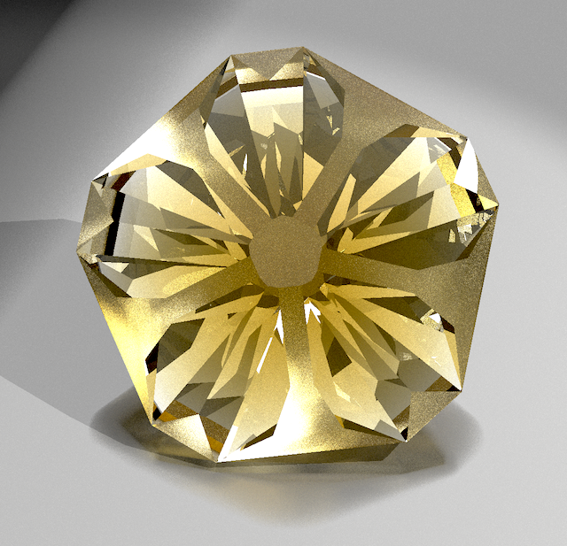
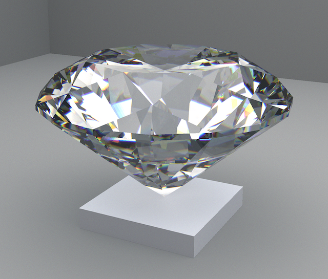
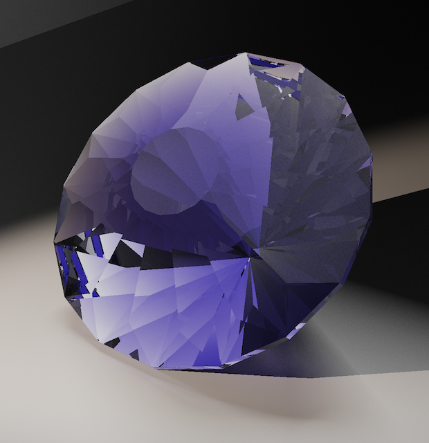
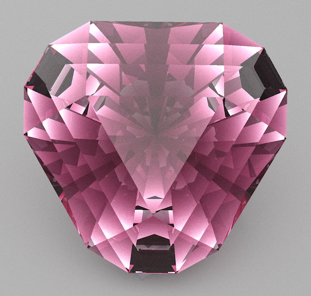
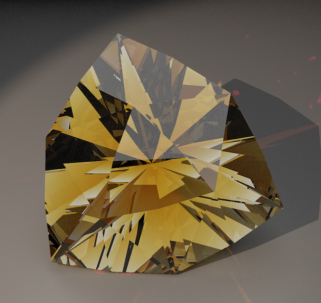
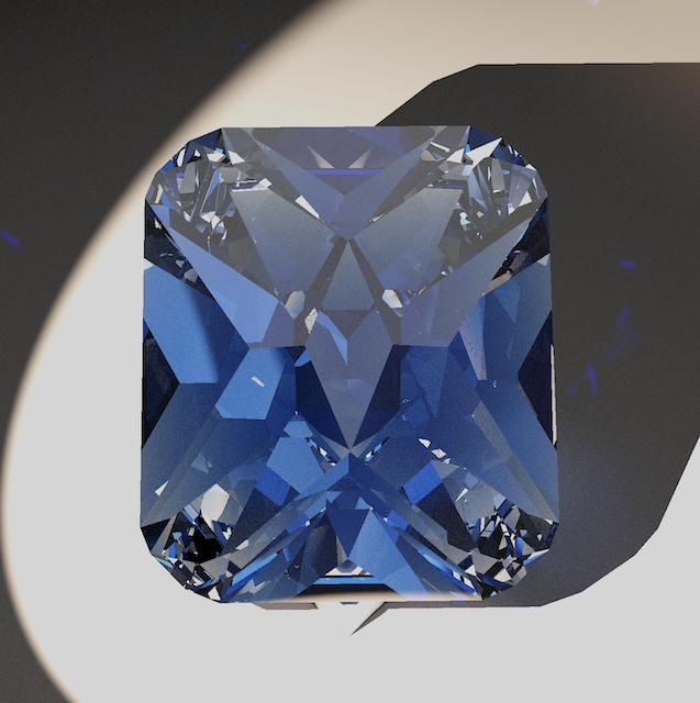
This image is made in ProFacet using the upcoming path tracer. Explore more designs in our Gallery.
Documentation Structure
Because the coding part is optional, we've organized the documentation into two parts:
- Part 1: The Studio covers the visual tools you need to design and cut. This is all you need to get the job done.
- Part 2: FSL Reference covers FSL, the powerful language underneath. It serves as an alternative to the UI, especially useful for precise manual adjustments or advanced parametric designs.
If you're interested in learning how to read or write the recipe directly, or want to use advanced algorithmic features, check out Part 2. Otherwise, feel free to stick to Part 1 and just cut!
Contact
If you have questions, feedback, or need support, join our Discord community.
Timeline
- Test Phase: now through 1 Mar 2026—iterate, gather feedback, and refine the tools and documentation while everything is still in flux.
- Contest Window: 1 Mar – 1 May 2026—run the launch performance contest and keep the Hobbyist tier free so every cutter can participate.
- Paid Phase: begins 1 May 2026—introduce billing for the Analyzer, Optimizer, Path Tracer and Cloud Sync. The "offline" mode without these tools will stay free to use.
Quick Start: Interactive Slicer
This quick start focuses on learning the Interactive Slicer by walking through the first pavilion tier, girdle, crown, and table. Keep the studio open in another tab so you can follow along.
Tip: The studio autosaves in your browser. Close the tab and come back later—your last design reopens automatically.
1. Open the studio and click New
Launching the studio drops you into the 3D stage. By default, the Interactive Slicer tab is active below the viewer (or to the side on large screens).
To see the code, switch to the Spec Editor tab. Hit New to load the blank template:
name = "Untitled Design"
ri = 1.54
gear = 96
This is the starting "rough" we’ll carve away.
2. Set up the first pavilion tier
Switch back to the Interactive Slicer tab if needed:
- Choose Pavilion for the side (we normally begin on the pavilion).
- Set Symmetry to
8. - Enter Angle
37.50°and Base Index0. - Pick Center Point (
cp()) as the target.
The slicing plane animates into view. Hovering over the Preview button displays the cut.
3. Commit the cut
Press Commit to apply the tier. The viewer redraws with the new facets. (You can verify the generated code in the Spec Editor tab):
name = "Untitled Design"
ri = 1.54
gear = 96

P1 0 @ 37.50 : cp() x8
Rotate the viewer and you’ll see the pavilion facets meeting at the center. More steps will follow, but getting comfortable with this rhythm—choose parameters, preview, commit—is the foundation for building complete stones.
4. Establish the girdle depth
Next, set up the girdle ring:
- Keep Side on Down, but change the Angle to
90.00°. - Switch the target to Depth and enter
1.00for the value. - Leave symmetry at
8and base index at0, then click Commit again.
name = "Untitled Design"
ri = 1.54
gear = 96

P1 0 @ 37.50 : cp() x8
G1 0 @ 90.00 : 1.0000
You now have the pavilion facets and the girdle defined—a solid foundation before working through additional tiers.
5. Cut the first crown tier
Now flip to the crown side:
- Change Side to Crown.
- Set Angle
25.00°, Symmetry8, and keep Base Index0. - Pick Proper Meetpoint as the target. The slicer will highlight multiple nodes—click the meetpoint where the girdle and pavilion facets touch.
- Check Girdle Offset so the cut keeps the girdle at the right thickness.
- Hit Commit to apply the crown tier.
name = "Untitled Design"
ri = 1.54
gear = 96

P1 0 @ 37.50 : cp() x8
G1 0 @ 90.00 : 1.000
C1 0 @ 25.00 : mp(P1, G1) + girdle
At this point, the pavilion, girdle, and first crown tier are in place.
6. Add the table
Finish the crown by cutting the table:
- Keep Side on Crown but change the Angle to
0.00°. - Select Depth as the target and drag the slider (or type) to your preferred table height.
- Set Symmetry to
1(tables are usually single facets). - Press Commit to flatten the top.
name = "Untitled Design"
ri = 1.54
gear = 96
size = 2.0
girdle = Vector(0, 0, 0.03)

P1 0 @ 37.50 : cp() x8
G1 0 @ 90.00 : 1.000
C1 0 @ 25.00 : mp(P1, G1) + girdle
T 0 @ 0.00 : 0.0900 x1
You now have a basic pavilion, girdle, crown, and table—enough to explore the diagram (printable instructions) or continue refining each tier.
What’s next?
- Open the Diagrams panel to generate printable SVGs once you finish a few tiers.
- Explore the Interactive Slicer guide in Tooling → Interactive Slicer for advanced targets and meetpoints.
Workspaces & Tools
ProFacet puts every workflow in the browser. These chapters explain what each panel does, why you might use it, and how the pieces work together.
- Web Studio - tour the editor, diagnostics, camera controls, and printable instructions.
- Analyzer - peek under the hood of the light-return charts and learn how to read them.
- Optimizer - understand the sliders, presets, and progress meters before you launch a run.
- Interactive Slicer - preview a candidate facet, inspect meetpoints, and drop the generated command into the editor.
- Symmetry Assistant - define and discover symmetrical patterns with forward and reverse modes.
- Launch Contest - submit designs for verification and track the community leaderboard.
- Cloud Sync & Accounts - optional online capabilities for sharing designs across devices.
- CAM Viewer - visualize and adjust Centerpoint-Angle Method system functions.
Browse in whatever order fits your session. Every walkthrough assumes you are using the live app and focuses on what you will see and click there.
Web Studio
Launch the browser studio (see Start Here) to get an editor, 3D viewer, printable instructions, and performance tools in a single workspace. Nothing to install - everything runs locally in your browser.
The workspace is organized into primary views (accessible from the sidebar) and tool tabs (within the 3D Studio view). By default, the 3D Studio view is active, showing the Interactive Slicer and Spec Editor tabs.
Editing workflow
[!NOTE] ProFacet requests persistent storage from the browser to keep your designs safe. Check About ProFacet to see if your storage is Protected or Standard — this is decided by the browser, not ProFacet. Either way, regular backups are a good idea: use Open → Backup to export a JSON file, and consider enabling Cloud Sync.
- Switch to the Spec Editor tab to write FSL code directly.
- The studio auto-saves shortly after you stop typing, keeping a private copy of every design in your browser.
- Use Open... to browse your saved designs, restore deleted entries, or export a JSON backup. New loads the default template.
- Errors and warnings appear directly under the editor with line numbers. Fix them before running the Analyzer or Optimizer - the performance tools stay locked until the last run succeeds.
Navigating the 3D viewer
- Rotate with a left-button drag (or a single-finger drag on touch).
- Pan with the right or middle button; on touch devices use a two-finger drag.
- Zoom with the mouse wheel or a pinch gesture. Double-click the canvas to reset the default view.
- Use the toolbar buttons to toggle overlays, reveal wireframe edges, display debug points, flip between crown and pavilion, or show the angle guide.
- Use the view mode dropdown to switch between Mono (Uniform), Palette, Raytraced, and BDPT (High-Quality Path Tracer).
The Interactive Slicer tab mirrors your current design: the panel slices the model, shows meetpoint indices, and reacts to Control/Cmd held down while you move the mouse for quick previews.
Printable instructions
Open Diagram to generate the same packet your printer will see:
- Pick a theme and image size (Small or Large) without leaving the studio.
- Toggle Compact to tighten table spacing, and have crown and pavilion side by side.
- Click Print to switch into a browser print preview; the rest of the UI hides automatically.
Performance tools
- Analyzer simulates 19 tilt positions on the GPU (see Analyzer for details). The panel stays disabled until the current design processes without errors and WebGPU is available.
- Optimizer adjusts every optimizable value, reuses the Analyzer scores, and keeps the best candidate ready for comparison (see Optimizer).
Both panels share the same Analyzer engine, so once WebGPU initializes successfully the buttons unlock together.
Launch Contest
Participate in the community performance contest by selecting Launch Contest from the sidebar. You can submit your design for verification, view the live leaderboard, and check the rules.
- Submissions require an active cloud session.
- Designs are scored automatically using the contest-specific weights.
- Only the design name and score are public during the contest.
Analyzer
Before you start
- Process the design first so the interpreter, viewer, and Analyzer are working on the same geometry.
- Clear every FSL error. The Analyzer is disabled until the last run finished without errors.
- The studio needs WebGPU and the Analyzer feature on your account.
Run an analysis
- Open a design and click Analyzer in the side bar.
- When the run finishes the metrics, charts, and timings update immediately.
Understand the results
- Metric cards list Average Brightness, Contrast Density, Contrast Intensity, Scintillation Score, and Compactness. Each value is shown as a percentage relative to the Hearts & Arrows brilliant reference that ships with the studio.
- Average Brightness is the mean return light over every valid pixel in the sweep.
- Contrast Density measures the amount of contrast areas visible on the stone. It describes the spatial distribution of light and dark zones.
- Contrast Intensity measures the strength of the contrast in areas where it exists.
- Scintillation Score counts blink events between angles and normalises them by the number of pixels and tilt steps.
- Compactness comes from the current mesh and reports how much of the stone's footprint-and-height envelope is filled by the actual volume.
- Shannon Entropy New! measures the information content or "richness" of the light distribution. A higher entropy score means the stone returns a complex, varied range of light levels—avoiding "flat" or monotone appearances.
- Per-angle sparklines ("Brightness by Angle", "Contrast Density", "Contrast Intensity") plot the same metrics for each of the 19 tilt angles so you can see where the stone rises or falls off.
- Lighting sweep renders each frame with cosine-weighted lighting and a standard head shadow. The 19 tilt positions start 45° down on the X axis, move through the upright view, and finish 45° toward the Y axis. Step sizes tighten near upright so more samples are taken where the stone spends most of its time, making every average a weighted view of the sweep.
Try it now
Paste the snippet below, process the design, and run the Analyzer to watch how tiny angle tweaks change the sparkline profiles.
name  = "Analyzer Demo"
gear  = 96

P1 0 @ 41.8 : 0.18 x8
P2 6 @ 39.6 : mp(P1) x8

G1 0 @ 90 : size x16
C1 0 @ 32.2 : mp(G1,P1) + girdle x16
T 0 @ 0 : 1.1
Optimizer
The Optimizer is the cornerstone of the ProFacet workflow and the feature that truly distinguishes it from other design tools. Uniquely enabled by the Facet Specification Language (FSL), it allows you to move beyond manual iteration and mathematically refine your design for peak performance.
By adding +/- hints to numeric values in your FSL script, you define a search space for the engine to explore. The Optimizer then leverages WebGPU acceleration to evaluate thousands of variations in real-time, scoring each one against professional-grade metrics for brightness, contrast, and scintillation. It is a seamless, powerful bridge between your creative intent and optical perfection.
Prepare adjustable values
- Add a
+/-hint after any numeric literal you want to expose:value +/- deviation. - The deviation can be absolute (
41.8 +/- 0.5) or a percentage (1.76 +/- 5%). - Hints work anywhere the interpreter accepts a literal: configuration commands, facet commands, function arguments, and expressions.
Example block ready for optimization:
name = "Optimizer Demo"
gear = 96

P1 0 @ 41.0 +/- 1.5 : 0.18 x8
P2 6 @ 39.5 +/- 1.5 : mp(P1)
P3 12 @ 38.2 : 0.16

G1 0 @ 90 : size x16
C1 0 @ 32.0 +/- 2.0 : mp(G1,P1) + girdle
T 0 @ 0 : 0.9
If no hints are present the engine returns "No optimizable parameters found" and stays idle.
Choose your weights
- Open the Optimizer panel with Open Optimizer.
- Pick a preset to load weights for Average Brightness, Contrast Density, Contrast Intensity, Scintillation Score, and Compactness. The built-in presets are Balanced Default, Brilliance Boost, Contrast Focus, Precision Cut, and 2026 Launch Contest.
- Adjust any slider between 0 and 10. Press Save Preset to store the current mix; the studio keeps a local copy and syncs it to your account when cloud features are available.
Launch and monitor a run
- Process the design and clear every FSL error. The Optimizer checks the same run status as the Analyzer and will show the reason if it stays locked.
- Press Start Optimization. The button switches to "Optimization Running", the cancel button becomes Stop & Keep Best.
- The progress panel lists the current status, iteration, best score (calculated from your weights on Hearts & Arrows-normalized metrics), analyzer throughput in pixels per second, and metric deltas versus the starting design.
- Stopping keeps the strongest candidate so far and turns the start button into Resume Optimization; you can pick up right where you left off without losing that snapshot.
- When you resume after stopping, the percent deltas still reference the very first score from that session—stopping does not reset the baseline. If you apply or save the optimized version to the editor, the next run treats that updated design as the new baseline.
Behind the scenes the Optimizer explores nearby combinations automatically and never strays outside the min and max you set.
Compare and apply
- As soon as a valid candidate exists the comparison panel opens with side-by-side viewports labeled Original and Optimized plus a contribution table that shows how each metric moved.
- The Replace Editor with Optimized button swaps the editor contents with the current best parameters. Save Optimized as New Version writes a revision while preserving the original file.
- Apply actions stay hidden until you stop a run. Resume after applying if you want to explore further from the updated baseline.
- Stopping caches the best parameters and the best score. Hitting Resume seeds the next run with that candidate so the population starts from where you left off instead of restarting from the original design. If you apply/save the optimized design first, the next run treats that new file as the baseline.
Interactive Slicer
The Interactive Slicer panel (the “Interactive Slicing” column under the Viewer) lets you preview a candidate facet, inspect the exact meetpoints it would hit, and then paste the generated FSL command into the editor with one click. It is powered by the same Renderer and meetpoint pipeline that the studio uses during normal execution, so the preview reflects the current geometry, symmetry, and girdle settings.
Panel layout

- Side – choose
Up(crown) orDown(pavilion). The side to cut. - Symmetry / Mirror – set the repeat count (
xN) and whether to emit mirrored pairs (xxN). The slicer syncs the starting value from the current machine snapshot; it only appendsx/xxto the preview command when you change it. - Target – selects what the facet should touch:
None (hide preview)disables all overlays and buttons.Center pointusescp(the center axis) and asks ProFacet for the exact center when context is available.Girdlereturns the girdle contact at the current index/angle using thegphelper.Proper meetpointpulls clustered meetpoints fromlistMeetpoints; use ◀/▶ to cycle through candidates.Depthexposes a depth slider (0–1.00) for classic angle + depth cuts. Check Optimizable to append+/- 5%, marking the depth for optimization.
- Angle / Index – slider + number pairs that map directly to the machine angle (0–90°) and index (0–gear). Drag the slider for coarse changes, or type numbers for precise edits. While the pointer is over the angle slider, hold
Ctrl(Cmdon macOS) to activate fine-grained mode. Use the Optimizable checkbox to append+/- 5%to the generated FSL, marking the angle for later optimization. - Girdle offset – when the target is
cp,gp, orProper meetpoint, adds+ girdleon the crown or-girdleon the pavilion automatically.
Below the controls you will see:
- A meetpoint navigator (visible only for
Proper meetpoint). Each candidate shows its label, order, and whether it is a fallback. When the selected point lies on the girdle, the preview command switches togp. - A live preview string that mirrors the facet command that would be added to the editor.
- The floating Preview badge, plus Cancel and Commit buttons.

Preview behavior
- Dragging the angle or index slider, hovering the Preview badge, or holding
Ctrl/Cmdkeeps the preview active. - The Viewer shows:
- A plane overlay and cap polygon sliced through the current mesh.
- Markers for the selected meetpoint (and neighbouring candidates), the current
cporgp, and any girdle candidate provided by ProFacet.- The angle guide if it is enabled in the Viewer.
- When you release the slider or let go of the modifier key, the preview snaps back to the base mesh.
Committing or cancelling
- Commit (
Shift+Enter) appends the preview line to the editor, choosing the next sequential tier name (P,C, orGbased on side/angle), and reruns the interpreter so the Viewer stays in sync. - Cancel clears the preview state and resets the target to
None.
Meetpoints
Proper meetpointfilters out fallback candidates and anything that falls on the opposite side of the plane. The panel remembers your selection as you change the angle or index.
Symmetry and warnings
- The symmetry count must divide the machine gear. If it does not (or if the index exceeds
gear / symmetry), the input fields highlight in red and a warning appears above the preview string. - Mirroring uses
xxand produces left/right pairs, matching the way the runtime interpretsxxN.
Tips
- Precision mode (
Ctrl/Cmdwhile the pointer is over the Angle or Depth slider) lets you make fine-grained adjustments without typing numbers. - Hold
Ctrl/Cmdwhile tapping arrow keys in the numeric boxes to keep the preview active. - The preview command already includes any
+ girdle, symmetry, or meetpoint specifier adjustments, so the inserted line is ready to run as-is. You can still edit it manually in the editor after committing if you need to tweak the tier name or add notes.
Symmetry Assistant
The Symmetry Assistant is a tool designed to help you define and discover symmetrical patterns for facet indexing. It provides two primary modes of operation: Forward and Reverse.
- Forward Mode allows you to specify symmetry parameters (symmetry count, index, and whether it's mirrored) and see the full list of resulting facet indices. This is useful when you know the symmetry you want to apply and need to visualize the result.
- Reverse Mode is a powerful predictive tool. You can type a few indices from a sequence, and the assistant will deduce the underlying symmetry parameters, complete the sequence for you, and even suggest alternative interpretations. This is invaluable when you have a partial pattern in mind and want to establish the full symmetrical loop.
Accessing the Assistant
The Symmetry Assistant can be opened from the user interface:
From the Interactive Slicer: A small "?" button appears next to the "Mirrored" checkbox in the main symmetry controls. Clicking this will open the assistant, pre-filled with the current settings from the widget.
When opened, the assistant syncs with the slicer's current gear count.
Core Concepts
Before diving into the modes, let's define some key terms:
- Gear: The total number of available index positions on the gear (e.g., 96 for a standard faceting machine).
- Symmetry: The number of times a pattern repeats around the gear. The
gearcount must be perfectly divisible by thesymmetrynumber. - Index: The base or starting index from which a symmetrical pattern is generated.
- Mirrored: If enabled, the pattern is reflected across the 0-axis. For every generated index
p, its negative counterpart-p(modulo the gear size) is also included. - Step: The distance between each symmetrical index. It is calculated as
Gear / Symmetry. - Base Offset: The effective starting index of the pattern, calculated as
Index % Step. - Indices: The final, sorted list of unique index positions generated from the symmetry parameters.
Forward Mode
Forward mode is for expanding a known symmetry into a full set of indices.
How to Use
- Open the Assistant: It will default to Forward mode.
- Enter Parameters:
- Index: Set the base index for the calculation.
- Symmetry: Set the desired symmetry count. This must be a divisor of the current gear count.
- Mirrored: Check this box to create a mirrored pattern.
- Review the Output:
- The assistant immediately calculates and displays the full list of
Indices. - Below the inputs, metadata is shown, including the calculated
step,symmetry,mirroredstatus, andbase offset. - If there's an error (e.g., "Symmetry must divide the gear"), a message will appear.
- The assistant immediately calculates and displays the full list of
- Apply the Symmetry:
- Click "Send to slicer" to apply the generated symmetry to the main application. The assistant will close, and the slicer's symmetry settings will be updated.
Example
With a gear of 96:
Index: 2Symmetry: 8Mirrored: false
The assistant calculates a step of 96 / 8 = 12. It generates the indices: 2, 14, 26, 38, 50, 62, 74, 86.
Reverse Mode
Reverse mode is for discovering symmetry parameters from a partial sequence of indices. It's like asking the assistant, "What symmetry creates a pattern that starts like this?"
How to Use
- Switch to Reverse Mode: Click the "Reverse" tab at the top.
- Enter a Prefix:
- In the "Indices prefix" field, start typing the first few indices of your desired pattern, separated by commas or spaces (e.g.,
2, 10). The indices must be in ascending order.
- In the "Indices prefix" field, start typing the first few indices of your desired pattern, separated by commas or spaces (e.g.,
- Review the Prediction:
- As you type, the assistant analyzes the prefix and finds the best-fitting symmetry parameters.
- Ghost Text: The input field shows a "ghost" completion of the full sequence based on the best prediction.
- Completion: The "Completion" box displays the full list of indices. The numbers you typed are locked, while the predicted numbers are clickable, allowing you to add them to your prefix.
- Next Number Chips: Below the input, clickable "chips" suggest the most likely next numbers to add to your sequence. This is useful for exploring different symmetry possibilities.
- Metadata: The predicted
step,symmetry,mirroredstatus, andbase offsetare displayed.
- Explore Alternatives:
- If your prefix can be interpreted in multiple ways, a section titled "Other interpretations" will appear.
- You can expand this section to see alternative symmetry solutions that also match your prefix. Clicking on an alternative's index list will preview it as the main solution.
- Apply the Symmetry:
- Once you are satisfied with a predicted sequence, click "Send to slicer". This applies the selected symmetry parameters to the main application.
Example
With a gear of 96, you type 2, 10 into the prefix field.
-
The assistant immediately predicts a mirrored symmetry of 8.
- Parameters:
step=12,symmetry=8,mirrored=true,base=2. - Completion: It shows the full sequence:
2, 10, 14, 22, 26, 34, 38, 46, 50, 58, 62, 70, 74, 82, 86, 94. - Ghost Text: Your input of
2, 10is followed by the ghost text, 14, 22, .... - Next Chips: It might suggest
14as the next logical number.
- Parameters:
-
At the same time, it might find an alternative: a non-mirrored symmetry of 12.
- Parameters:
step=8,symmetry=12,mirrored=false,base=2. - Completion:
2, 10, 18, 26, 34, 42, 50, 58, 66, 74, 82, 90. - This will be listed under "Other interpretations".
- Parameters:
Scoring Model
The score is a weighted sum of five well-defined metrics. Contrast density and contrast intensity combine into a single contrast term because strong contrast requires both; the remaining terms are linear for clarity.
What goes in
- Metrics — Average Brightness, Contrast Density, Contrast Intensity, Scintillation Score, Compactness, and Shannon Entropy. Each is compared to the Hearts & Arrows reference; values above 1.0 mean “better than the reference”.
- Weights — The six sliders (
averageBrightness,contrastDensity,contrastIntensity,scintillationScore,compactness,shannonEntropy). Weights are always treated as zero or higher.
How the score is built
-
Normalize the metrics
Everything is turned into a ratio vs the reference. If a metric is better than the reference, we keep it above 1.0 but gently squash it so runaway values don’t dominate. -
Make contrast a single value
Contrast density and intensity are blended with a geometric mix (think “both must be good, one can’t carry the other”). If both contrast sliders are equal, this behaves like the square root of (density × intensity). If one slider is higher, that side is favored—but a weak partner still drags the contrast term down. -
Set the overall weights
The two contrast sliders also decide how important contrast is overall: their average becomes the contrast weight. Brightness, scintillation, compactness, and contrast weights are then scaled so they always sum to 1 (extras are included the same way). -
Take the weighted sum
Final score = brightness part + contrast part + scintillation part + compactness part. Higher numbers mean closer to, or better than, the reference cut.
Notes
- The contest verifier, Optimizer, and UI all share this exact formula, so what you see is what gets verified.
Cloud Sync & Accounts
ProFacet stores every edit in your browser first for speed and data privacy. Cloud sync builds on that foundation: when you sign in, the studio mirrors those designs to your account so you can pick up the same work on another machine. This chapter explains what stays local, what changes after authentication, and how to keep multiple browsers aligned.
Local storage and manual backups
ProFacet requests persistent storage from the browser at startup to keep your designs safe. If granted, your data is labelled Protected — the browser guarantees it will keep your data even when disk space is low. If not granted, your data is labelled Standard — everything works the same, but the browser may clear site data if the disk runs very low.
[!NOTE] Whether storage is Protected or Standard is decided by the browser, not by ProFacet. Most browsers grant persistence for sites you visit regularly, bookmark, or install as a web app. You can check the current status in About ProFacet (click the ProFacet logo in the sidebar).
Either way, your designs are saved locally and work the same. Regular backups are still a good idea in case you ever clear site data, switch browsers, or move to a new machine:
- Open Design → Backup exports the entire library (active and deleted designs) as a JSON file you can keep on an external drive, in cloud storage, or anywhere you like. Restoring that file walks you through conflicts: you can overwrite locals with the backup or keep whichever version has the newest change.
- Cloud Sync automatically mirrors every design to your account so you can recover on another device (see below).
- Deleted entries stay two weeks in the dialog's Deleted filter until you purge them or restore them, so accidental removals are easy to undo.
- Always keep multiple backups (cloud sync, JSON export, external drive) so you can recover if anything goes sideways.
Signing in unlocks cloud sync
Click the Sign In badge in the editor header to open the account menu. Depending on the deployment, cloud features may be disabled entirely - in that case the badge simply reads Offline and behaves like a label.
When cloud sync is available, authenticating adds:
- Automatic backups - the latest copy of every design is stored alongside your account.
- Cross-device libraries - any browser that signs in with the same account receives the same portfolio. Remote designs win when they have a newer modification timestamp; otherwise your local edits stay in place.
- Preset sync - user-created optimizer presets are uploaded alongside designs, so the Optimizer panel shows the same list everywhere.
- Account controls - the menu offers Account Overview, Sync Now, Resend verification email (when needed), Delete Account, and Sign Out. Signed-out users get a one-click option to authenticate.
How syncing behaves
- Initial merge - the first sign-in pulls any remote snapshot, combines it with your local designs (newer changes win), saves the result back to the browser, and, if nothing is open, loads the most recently edited piece.
- Deferred uploads - after you edit a design, the badge notes that changes are waiting. About 45 seconds after you stop typing, the studio pushes the updated library so quick tweaks batch together.
- Interval syncs - while you are signed in, the studio also refreshes your cloud copy roughly every 10 minutes in the background.
- Manual Sync Now - choose Sync Now from the profile menu to force an immediate round-trip before you close a laptop or switch machines. The menu closes once the request completes.
- Optimizer presets - the presets you create travel with your account, so the Optimizer panel shows the same list wherever you sign in.
If the network is unavailable, sync retries later and your edits remain in IndexedDB. The spinner disappears once the controller falls back to idle.
Troubleshooting
- Designs are missing after signing in - open the profile menu and run Sync Now once to trigger a merge. If the designs still do not appear, check the browser console for
[cloud-sync]errors. - Contest submission says email unverified - use the menu's Resend verification email action and complete the link in your inbox, then try again.
- Preparing to wipe a device - export a JSON backup first (
Open Design -> Backup). You can restore that file on the fresh install before or after you sign in.
Sharing a Design
The goal of this feature is simple: share any design with anyone by sending them a single URL. The entire design is encoded directly into the link—no accounts, no file uploads, no server needed. The recipient clicks the link and sees your design instantly in ProFacet.
How It Works
When you click Share, the app takes the current FSL source and metadata (name, timestamp) and encodes it into a ?fsl= URL parameter. The result is a self‑contained link you can paste into a chat, e‑mail, forum post, or anywhere else. Nothing is uploaded to a server; the design lives entirely inside the URL.
Creating a Share Link
- Open the design you want to share. The link captures the current editor buffer, not the last saved version.
- Click Share in the upper toolbar. A panel appears with the link, and it is also copied to your clipboard automatically.
- Send the link. Anyone who opens it will see your exact design.
What the Recipient Sees (Scratch Mode)
When someone opens a shared link, the workspace enters scratch mode—a read‑only preview that protects both your work and theirs:
- The editor shows the shared design but editing is disabled. Typing, running the optimizer, opening files, and keyboard shortcuts are all blocked.
- A yellow banner at the top explains that this is a read‑only shared design.
- Two buttons appear in the toolbar: Copy to Library and Cancel.
This ensures the recipient gets a clean view of the design without accidentally overwriting anything in their own workspace.
Keeping or Dismissing the Design
Copy to Library
Click Copy to Library to save the shared design as your own:
- The design is persisted locally with its original name and metadata.
- Scratch mode exits, the
?fsl=parameter is removed from the URL, and all controls are re‑enabled. - From here you can rename, edit, optimize, or re‑share the design like any other.
If the save fails (e.g. IndexedDB is disabled), the workspace stays in scratch mode so you can retry.
Cancel
Click Cancel to dismiss the shared design without saving. Your normal workspace is restored exactly as it was.
Tips & Limitations
- Privacy: shared links are client‑side. Anyone with the link can read the FSL in the URL, so avoid posting sensitive work publicly.
- Size limit: very large designs may exceed URL length limits and fail to encode.
- Re‑sharing: after copying a design to your library you can re‑share it at any time—the Share button always reflects the current buffer.
CAM Viewer
This interactive tool allows you to visualize the various CAM (Centerpoint-Angle Method) system functions available in ProFacet. You can adjust the parameters to see how they affect the preform shape.
Select a shape from the dropdown and tweak the parameters. The viewer shows the result as a 3D mesh, defaulting to a pavilion view (looking from the bottom) to inspect the outline.
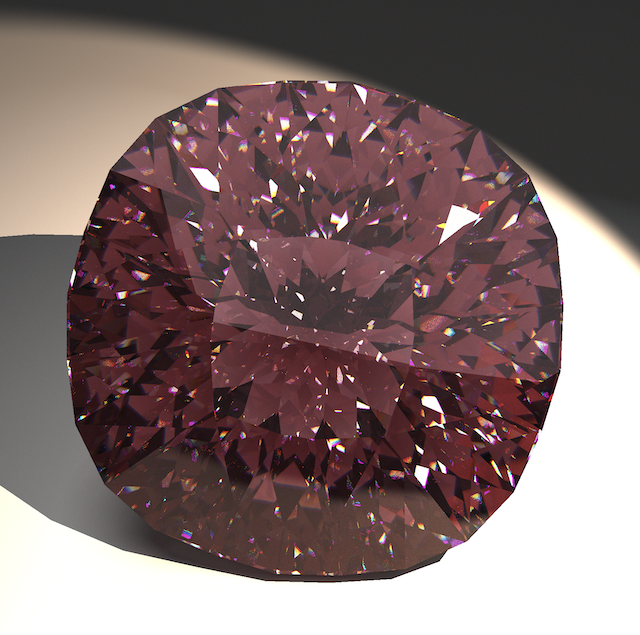
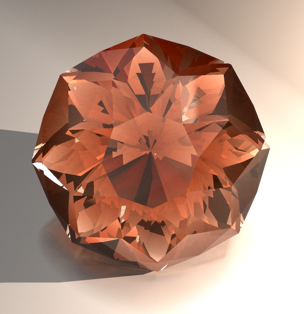
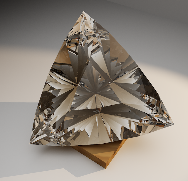
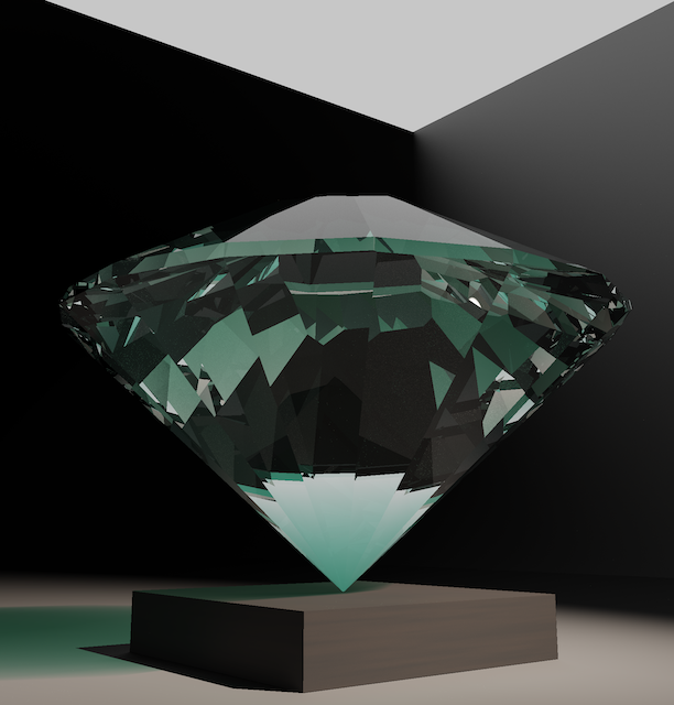
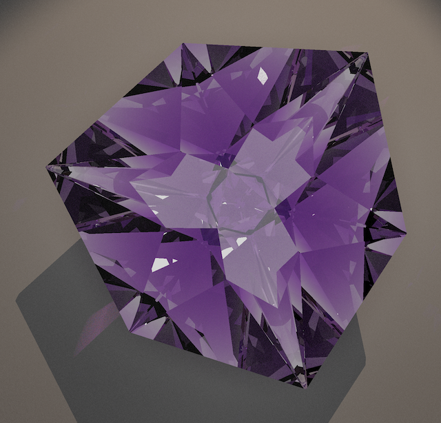
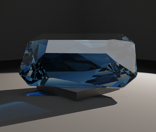
Gallery 1
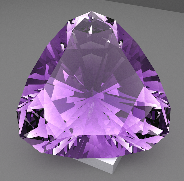
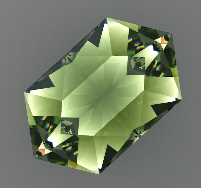
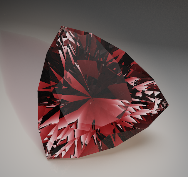
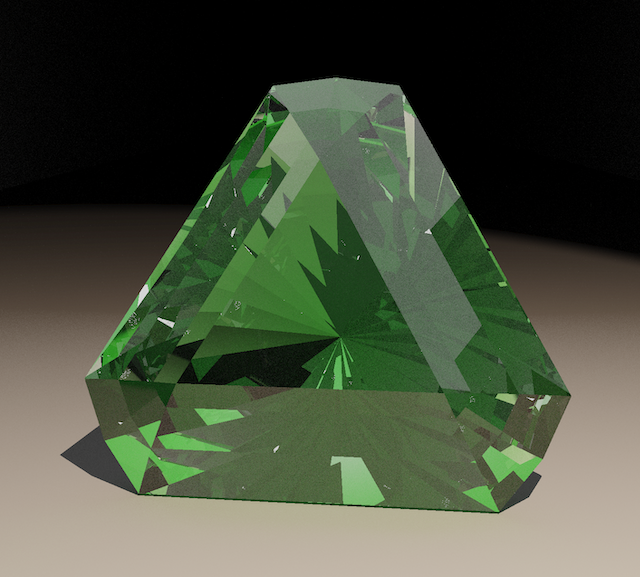
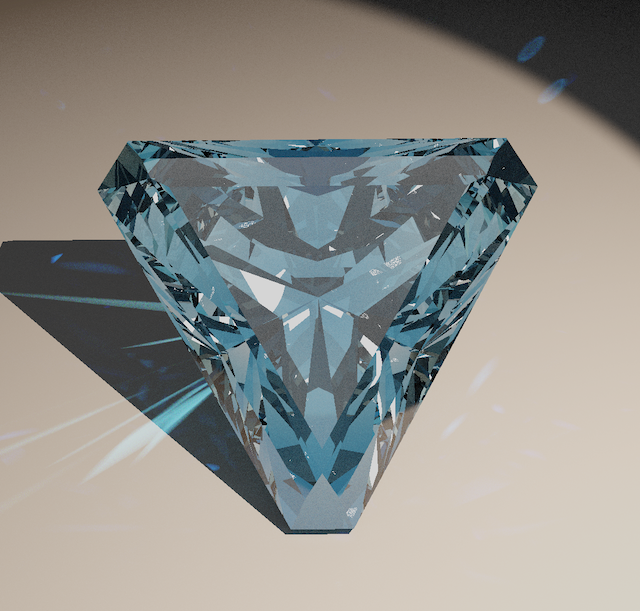
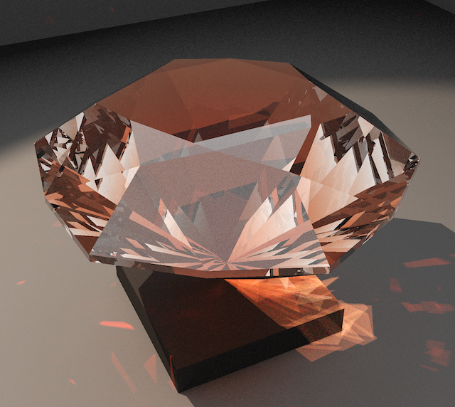
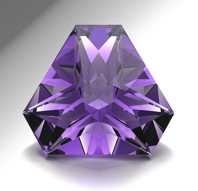
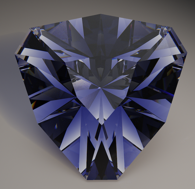
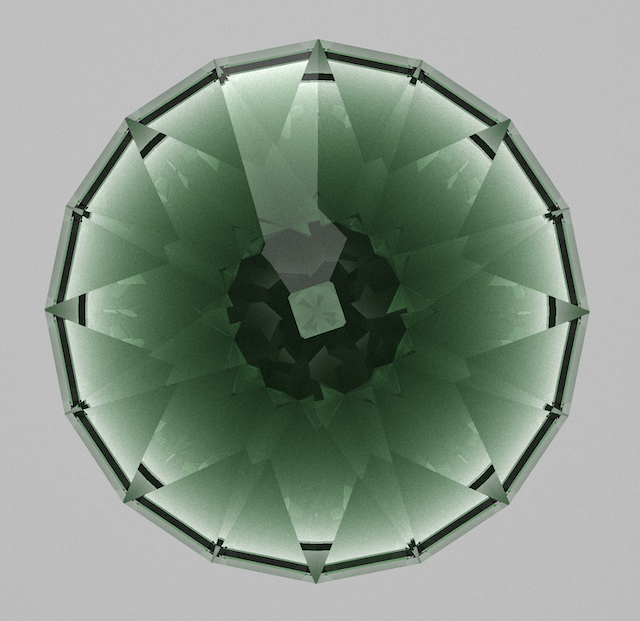
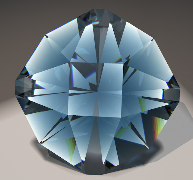
Work in progress. These images are generated with our bidirectional path tracer, which is still being worked on. The path tracer is a physics-based renderer that uses Monte Carlo sampling to approximate the full light-transport solution: many random rays per pixel, many bounces, and progressive accumulation until the image converges. The stones are shown in a simple light box with even top lighting and optional spot light. No head shadows or special effects, just aiming for a realistic image.
Image quality varies. The renderer is under active development, so older images may look less good than newer ones, e.g. due to simple caustics.
 Sakura 96 by Marco Voltolini |  Beginner Trillion by Michiko Huynh |
 Rubicello- Marco Voltolini |  Void Reaver by Arya Akhavan |
 Standard Round Brilliant Cut with fire (dispersion) |  Step Cut |
 Princess Cut on brushed aluminum |  Step Cut |
 Crisantemo by Marco Voltolini | 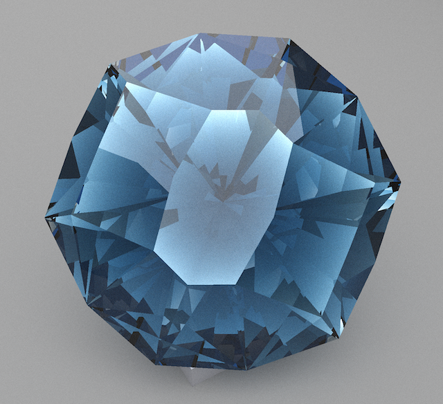 Abyssal Maw - Arya Akhavan |
 Voltolini-Tristano | 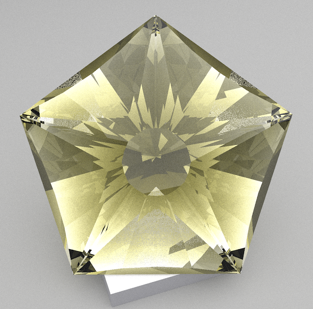 Akhavan-FallenStar |
 FVS-336 Trillium | 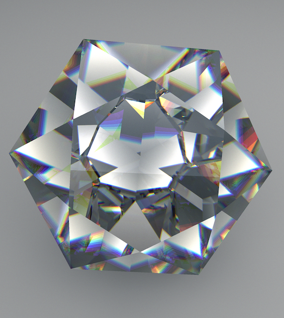 2014 Maximize Entry 6 Marco Voltolini |
 Laborie - One Rupee | 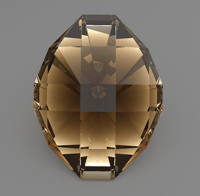 Bug Barion - Marco Voltolini |
 SRB with spot light | 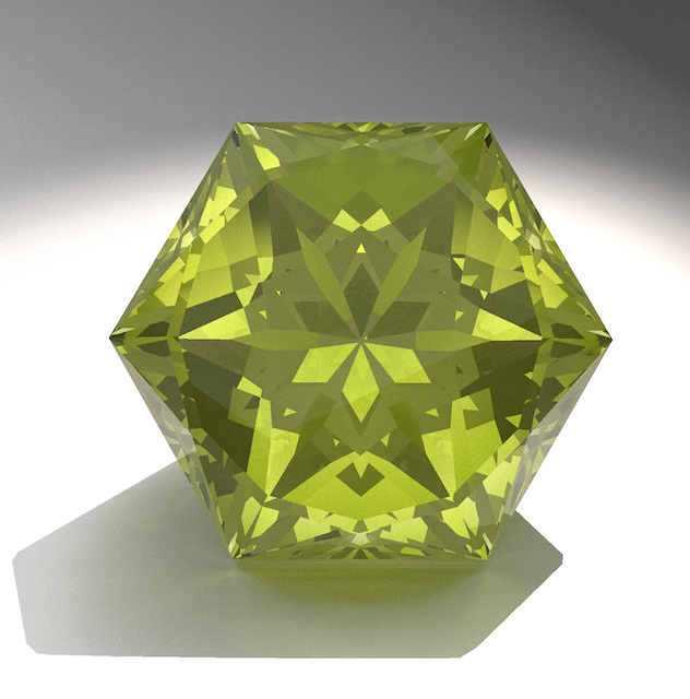 Frost Star Hex - Andrew Brown |
 FVS-162 Modified Orion - by Fred W. Van Sant | 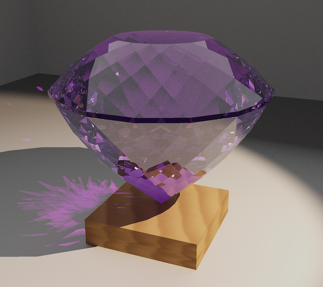 Portuguese Cut |
Gallery 2
Image quality varies. The renderer is under active development, so older images may look less good than newer ones, e.g. due to simple caustics.
 Blinder - Tom Herbst |  Hanami - Marco Voltolini |
 Akhavan – Heavens-Piercing Drill | 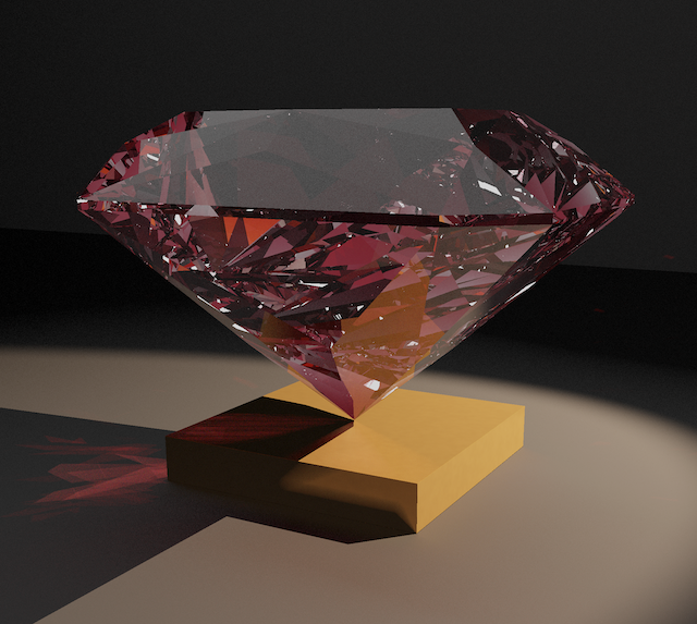 FVS-90 on copper |
 Star Trek Trillion - Jim Perkins | 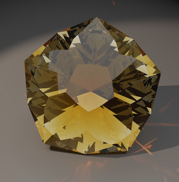 Fiorello 80 - Marco Voltolini |
 Tribal- Marco Voltolini | 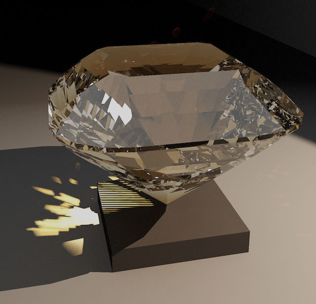 FVS-145 |
 FVS-80 | 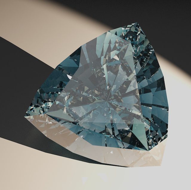 Signature#4 - Jeff Graham |
 Fancy Hexagonal Brilliant, by Jim Perkins | 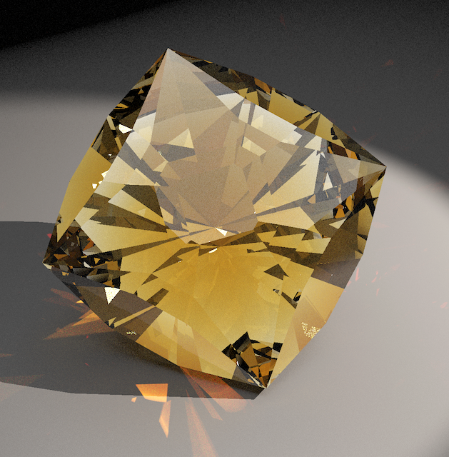 Hoshi - Marco Voltolini |
Next: ProFacet Designs → ← Previous: Gallery
ProFacet Designs
Designs by ProFacet's designer
 ProFacet-1 |  ProFacet-2 |
 ProFacet-3 | 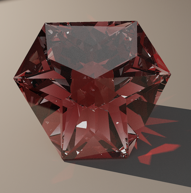 ProFacet-4 |
 ProFacet-5 | 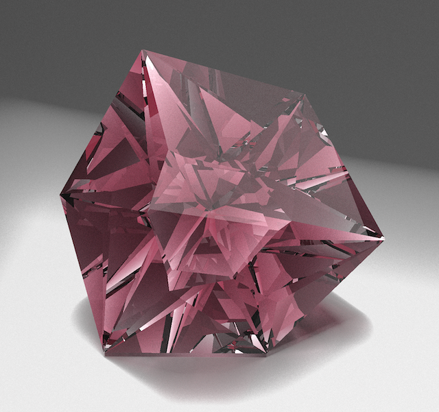 ProFacet-6 |
 ProFacet-7: Mesmerizing | 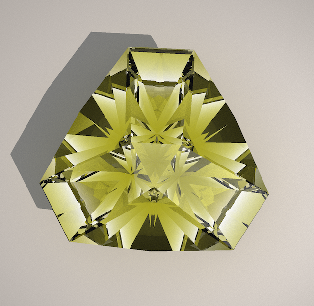 ProFacet-8 |
 ProFacet-9 | 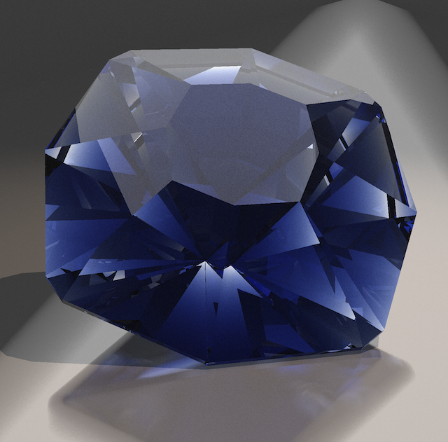 ProFacet-10 |
 ProFacet-11 | 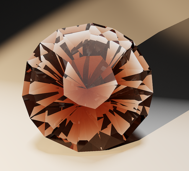 ProFacet-12 |
 ProFacet-13: Claude enters the chat | 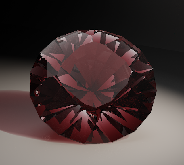 ProFacet-14 |
 ProFacet-16 | 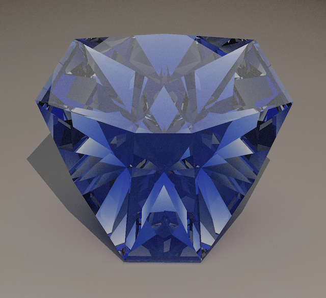 ProFacet-17 |
 ProFacet-18 | 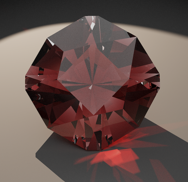 ProFacet-20 |
 ProFacet-21 | 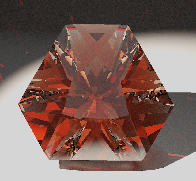 ProFacet-23 |
 ProFacet-24 | 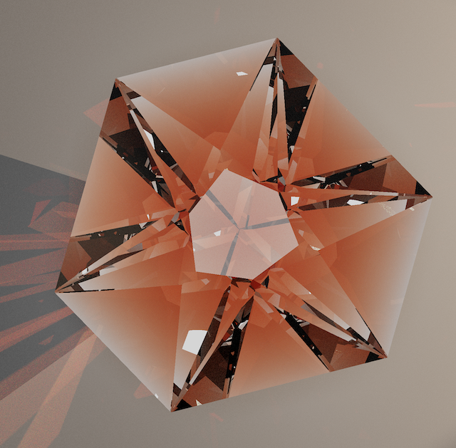 ProFacet-25 |
 ProFacet-26 |
FAQ
Q: Can I import .gem, .asc, .gcs, or .fsl files?
A: Yes—there’s an experimental importer in the workspace menu (the three-line “hamburger” next to Process) that accepts those formats. It tries to reverse-engineer the topology (which tiers connect, how symmetry repeats, which meetpoints matter) from mostly geometric data. That reconstruction is heuristic: it works surprisingly well on many files, but it’s not perfect, and the importer will spell out what it could or couldn’t infer in the generated FSL.
Q: Why can’t I manually inspect light rays and adjust windowing?
A: Modeling every ray and every facet angle by hand is practically impossible—slight changes ripple through the entire stone, and no one can cover those consequences better than the machine. We lean on our GPU-powered computation because it outperforms manual tweaking, letting you spend energy on the actual design decisions instead of endlessly chasing individual rays.
Q: Why does ProFacet lean on WebGPU for its heavy compute passes instead of sticking to CPU or WebGL?
A: Optimization sweeps, lighting analyses, and the raytraced preview all boil down to parallel math: tracing millions of rays, sampling BRDFs (models that describe how light reflects off a material), and updating facet energy buffers every frame. WebGPU unlocks dedicated compute pipelines, storage buffers, and subgroup ops, so we can keep those workloads on the GPU without round-tripping through JavaScript. Trying to express that in WebGL would mean abusing fragment shaders and multiple render targets, which is slower, harder to debug, and far less predictable across drivers.
Q: How do I know whether my browser (or GPU driver) supports WebGPU today?
A: Visit caniuse.com/?search=webgpu and scroll down to the support matrix. Green boxes indicate native support; yellow entries usually require enabling an experimental flag in chrome://flags, edge://flags, or the equivalent in Safari Technology Preview. Red entries mean WebGPU is still unavailable on that platform, so plan on updating your browser or OS before relying on it for production work.
Q: I have P1 42.00 08-12-16-32-36-40-56-60-64-80-84-88, but the Symmetry Assistant says it isn’t valid. What’s wrong?
A: That string actually represents two symmetry loops interleaved together, so the assistant can’t guess a single pattern from it. Split the data by alternating indices: P1 42.00° 8, 16, 32, 40, 56, 64, 80, 88 and P2 42.00° 12, 36, 60, 84. Paste each loop separately and the Assistant will happily detect the symmetry for both tiers.
Q: Is this using a proper geometric modeling CAD kernel?
A: Yes. ProFacet runs on a Swiss Made 🇨🇭 precision kernel purpose-built for CAD workflows. It uses arbitrary-precision floating point math, so no drift creeps into the model—even under deep zooms or long optimization passes—keeping every point exactly where it belongs.
Q: Can I export the rendered mesh as a Wavefront .obj file?
A: Yes. Process the design first so the viewer has a current mesh, then click the hamburger button next to the Process chip and choose Export OBJ. ProFacet generates a watertight mesh straight from the WASM buffers, names the file after your design (or profacet-model.obj if unnamed), and downloads it immediately so you can inspect or 3D-print the model in other tools.
Q: How do I contact support or give feedback?
A: Join our Discord community for questions, feedback, and design discussions. Use #help for support, #bug-reports for bugs, and #feature-requests for suggestions.
Q: Is there a way to auto format FSL source inside the editor?
A: Focus the FSL editor and press Ctrl+Shift+F (or Cmd+Shift+F on macOS) to run the formatter so spacing and delimiters are normalized automatically.
Community
ProFacet has a Discord server where faceting enthusiasts share designs, ask questions, and discuss optimization strategies.
→ ProFacet Discord{target="_blank"}
Channels
| Channel | What it's for |
|---|---|
#general | Introductions and general discussion |
#show-your-designs | Share renders, screenshots, and FSL code |
#fsl | Discuss the FSL language — syntax, patterns, and tricks |
#help | Get help with ProFacet, FSL, or gemstone design |
#launch-contest | Discuss the launch contest, compare strategies, celebrate winners |
#feature-requests | Suggest new features or improvements |
#bug-reports | Report bugs you've found |
Guidelines
- Be respectful — constructive feedback only.
- Stay on topic — use the right channel for your message.
- Share freely — post your designs, code, and renders. The community learns from each other.
- No spam — no self-promotion outside the designated channels.
Privacy, Ownership, and Simulation Disclaimer
Cookies and tracking
- We do not use third-party cookies, analytics pixels, or advertising trackers.
- Session cookies stay first-party (scoped to
profacet.com) and exist only to keep you signed in when you opt into account features.
Design ownership
- Your designs remain yours. We do not mine, resell, or reuse them.
- Designs are only shared outside your account when you submit them to an official contest.
Hosting and infrastructure
- ProFacet is hosted on Firebase (Google Cloud). Think of it as renting a secure storage unit: we control the keys and decide what lives there.
- Security-sensitive services—authentication, encryption at rest, and access controls—run on Google Cloud’s managed stack, so they inherit the same hardened protections Google applies to its own infrastructure.
- Firebase serves the app over our own domain, so it does not drop third-party cookies or inject ads—everything you load still counts as first-party traffic.
- When you enable cloud sync, the files you pick are stored in Firebase solely so you can reach them from another device. Firebase acts as our subprocessor and cannot repurpose that data.
- Plain-language version for non-technical folks: we use Google’s servers the way you might use a bank vault. They keep the lights on, but they do not get to open the box, copy your designs, or sell your activity.
Payments and billing
- All subscriptions and checkout flows run through Stripe, a PCI Level 1 compliant payment processor trusted by millions of businesses.
- Stripe handles your payment info directly; ProFacet never stores card data. We only receive subscription status and minimal metadata needed to operate your account.
- Stripe encrypts and vaults cards, monitors fraud, and provides a customer portal so you can update or cancel billing anytime.
- If you have billing questions or want your payment data removed from Stripe, contact us and we’ll help route the request.
Storage model
- Projects live in your browser first. They stay local unless and until you enable cloud sync.
- ProFacet requests persistent storage from the browser at startup to keep your designs safe. If granted, your data is labelled Protected and the browser will keep it even when disk space is low. Otherwise it is labelled Standard, which means the browser may clear site data if the disk runs very low. This is decided by the browser, not by ProFacet. You can check the current status in About ProFacet.
- Regular backups are a good idea in case you ever clear site data or switch machines. Use Open → Backup to export a JSON file and/or enable cloud sync.
- Cloud sync mirrors exactly the files you pick to your account so you can retrieve them on another machine; disable it and no further uploads occur.
Simulation disclaimer
- The Renderer, Analyzer, and Optimizer are sophisticated simulations, but they are still simulations.
- Real stones will deviate because of polishing, material tolerances, lighting, and refractive index variance, so treat virtual results as guidance rather than a guarantee of optical performance.
Introduction to FSL
Welcome to the engine room!
ProFacet's visual tools are powerful and sufficient for creating complete designs. However, FSL (Facet Specification Language) is the underlying "recipe" that describes your gemstone design.
You can create any design without writing a single line of FSL. The Studio writes it for you as you interact with the slicer.
So why learn FSL? It serves as a powerful alternative to the UI. It is particularly convenient for:
- Manual Adjustments: Quickly tweaking angles or indices without clicking through menus.
- Precision: Defining exact mathematical relationships between facets.
- Automation: Creating parametric designs that adapt to different sizes or materials.
This part of the documentation contains all the technical details for FSL:
- Language Guide: Core concepts, syntax, and commands.
- Examples: Full FSL code for various cuts.
- Advanced Topics: Functional programming, parametric designs, and more.
- System Functions: Reference for built-in shapes.
FSL Tour
The Faceting Specification Language (FSL) is the handful of commands you type inside the studio to describe a cut, the toolbox you fall back on when the Interactive Slicer runs out of road. Most designs come together entirely in that panel, but intricate meetpoint choreography or exotic girdles go faster when you edit the FSL source directly. Once you get comfortable, you may find yourself jumping straight into the editor—experienced cutters often do because it is the quickest way to iterate.
Work through the chapters in order or jump to the one you need:
- Core Concepts explains how the studio reads an
.fslfile, what “up” and “down” mean, and how state carries from line to line. - Statements shows the building blocks—configuration (gear, ri, etc.), variables, facet commands, functions—each with short examples you can paste directly into the studio.
- Expressions covers numbers, point helpers, and the handy math functions you will reach for when lining up meet points.
- Functional Programming teaches you how to use this advanced feature to package repeated steps, especially for complex gem outlines.
- Facets and Tiers connects statement syntax to what actually happens to the stone.
The snippets are arranged so you can copy them into a new file, hit Process, and see the result immediately.
Core Concepts
Before we dive into individual commands, it helps to understand how the studio reads an .fsl file. Think of the interpreter as a very patient cutter: it reads a line, applies the change, then moves to the next line without skipping ahead or rearranging anything.
How the studio reads your file
- The file is a simple list of statements. Each line happens in the order you write it.
- Blank lines and comments are ignored, so feel free to add notes with
//whenever it helps future-you.
Here is a tiny program you can try in the FSL playground or copy and paste it into the studio to see it in action:
name = "Order Matters"
size = 1.0
gear = 96
girdle = Vector(0, 0, 0.03)

P1 0 @ 45 : cp() x4
G1 0 @ 90 : size
C1 0 @ 28 : mp(P1, G1) + girdle    // Depends on G1 and P1 already existing
T 0 @ 0 : 0.2 x1
The crown (C1) tier uses a meet point created by P1 and G1, so the line with the crown tier must come after P1 and G1.
What the studio remembers for you
While it reads the file, the studio tracks a handful of details in the background:
- Stone metadata –
name =,tags =,ri =, and friends. - Machine setup –
gear = 96; cw = truesticks until you change it, so every later facet uses the same gear and rotation. - Variables – Assignments store numbers or points that you can reuse later.
- Last side and symmetry – if you cut a pavilion facet (
down) and the next line starts with a tier name, the interpreter keeps usingdownunless you say otherwise. Same story for symmetry; once you typex8, the next cut command will also use that symmetry unless you change the modifier.
If anything goes wrong—maybe a meet point cannot be found—the interpreter stops right there and the diagnostics panel shows the line and message.
Crown versus pavilion
downfacets belong to the pavilion and tilt toward negative Z.upfacets belong to the crown and tilt toward positive Z.- Tier labels are just names.
P1,C1,Break, andStarall work.
Symmetry in plain language
Add xN after a facet command to copy it around the stone every 360 / N degrees. Use xxN when you want mirrored N-fold symmetry (each pair becomes a left/right mirror). The count must be a positive whole number:
P1 12 @ 38.2 : 0.16 x8           // eight pavilion mains
G1 0 @ 90 : size x16             // sixteen girdle facets (90°)
If you are cutting something asymmetric, you can skip symmetry entirely by spelling out every index in brackets: P1 [3, 27, 44] @ 90 : size hits those three teeth in order and stops. Because you already provided the full list, you do not add an x4 (or any other symmetry modifier) on that line. The first number in that bracket list still serves as the base index for helpers such as mp()/gp().
Numbers, points, and edges
Most expressions boil down to one of three value types:
- Number – plain angles, depths, or calculations like
Math.toDegrees(0.5). - Point – created with helpers such as
mp(P1),gp(), orPoint(0, 0, 1). These mark locations in space, whether pulled from existing facets or stated outright. - Edge – less common but handy for advanced functions, created with
edge(tier:index, tier:index).
You can store numbers or points in variables. Edge helpers always produce an array of two points, so capture the array and access points by index:
name = "Edge Example"
size = 1.0
gear = 96
girdle = Vector(0, 0, 0.03)

P1 0 @ 45 : cp() x8

pt1 = mp(P1)
print("Point 1:", pt1)

e = edge(P1:0, P1:12)
first = e[0]
second = e[1]
print("Edge endpoints:", first, second)

C2 up 0 @ 29.5 : pt1 + girdle x16
Variables live until the end of the file (or until a function finishes, if you are inside one).
With these basics in mind, continue to Statements to see every command you can type.
Statements
Every line in an .fsl file starts with a command, variable assignment, or tier name. The parser treats newlines as whitespace, so you are free to split long commands across multiple lines or use indentation for clarity. If you want to chain multiple statements on the same line, you must use a semicolon ; to separate them. This chapter explains what each statement does and why you would reach for it.
configuration (gear, ri, etc.) – project-wide settings
Use configuration assignments (gear, ri, etc.) to update metadata (name = "...", ri = ...) or machine configuration (gear = ...). The change applies immediately and carries forward to later lines.
| Command | Value syntax | What it controls |
|---|---|---|
name = "Brilliant Oval" | Quoted string | Updates the project title used in the Viewer, Analyzer panels, and printable exports. |
ri = 1.760 | Plain number or optimizable literal (for example 1.76 +/- 5%) | Defines the refractive index the Renderer, Analyzer, and Optimizer use for light calculations. |
color = "#ffd166" | Hex literal (#ffd166) | Sets the simulated material color in raytraces. |
notes = "..." | Quoted string | A text note to describe the design. |
tags | String list | Comma or space separated keywords (e.g., "round, brilliant" or "quartz green") used for searching in the file dialog. |
absorption | Number | Sets the absorption strength for the visual raytracer. Values around 1 look quite natural, but it depends on the color as well; higher values darken the stone. |
gear | Positive integer | Sets the index gear tooth count for every later facet. |
cw = true | Boolean (true for clockwise, false for counter-clockwise) | Sets the dop rotation direction. |
cube = 3.0 | Number interpreted as the cube’s edge length | Rebuilds the starting blank as a cube of the given size. Useful when you need extra “rough” after running out of material mid-cut. |
Assignment – save a value for later
pt = mp(P1) stores a point or number in a variable named pt so you can reuse it further down. Inside functions, the variable disappears when the function finishes; elsewhere, it is available until the end of the file.
Note: FSL uses direct assignment (
x = 10). Keywords likelet,const, orvarare not supported.
Need a list of numbers? Wrap them in brackets to build an array literal: angles = [41.8, 43.0, 32.2]. Every element can be any numeric expression—including optimizable literals such as 41.8 +/- 0.1—and the interpreter remembers the evaluated values at the moment the line runs. Read a value back with zero-based indexing (pavilion = angles[0]), and the interpreter will flag an error immediately if you stray outside the array’s bounds.
The edge(...) helper returns an array containing two points: the start and end of an edge. You can assign this array to a variable and access the points using zero-based indexing.
name = "Edge points"
gear = 96

P1 0 @ 41.8 : 0.18 x8

e = edge(P1:0, P1:12)
start_point = e[0]
end_point = e[1]

print("Start:", start_point)
print("End:", end_point)
Those bindings behave like any other point variable—you can aim facets at them, drop debug markers, or pass them into functions.
show – drop a marker in the viewer
show(mp(P1)) drops a marker using the default highlight color (#ff0000). You can supply a custom color as a second argument: show(mp(P1), "cyan") or show(mp(P1), "#ffe422").
The function accepts any number of points and colors. If a color string follows a point, it applies to that point.
name = "Show markers"
P1 0 @ 41.8 : cp() x8
// Mark the meet point in red
show(mp(P1), "red")
If you need to verify an edge, you can display its endpoints:
name = "Show Edge"
P1 0 @ 41.8 : cp() x8

// P1:0 and P1:12 are adjacent facets (steps of 12)
e = edge(P1:0, P1:12)

show(e[0], "orange")
show(e[1], "orange")
print – log values to the console
print statements are the quickest way to inspect a calculation. The interpreter prints the evaluated values to the browser/CLI console. It accepts multiple arguments and joins them with spaces. Examples:
name = "Debug example"
gear = 96

P1 0 @ 41.8 : 0.18 x8

angle = 41.8

print("entry point:", mp(P1))
print("angle offset:", Math.toRadians(angle) - 0.08)
print(ep(edge(P1:0, P1:12), 0.5))
Open your browser’s developer console (or the CLI output when running the interpreter directly) to see the output.
return – halt execution
Use return; at the top level to halt the interpreter immediately while keeping everything it has done so far: gemstone geometry, variables, debug markers, and the cut log. It is a handy escape hatch when debugging—pair it with show/print, inspect the partial stone, and keep experiments below the return; line without running them.
name = "Return demo"
P1 0 @ 41.8 : 0.18 x8
return;
P2 0 @ 43 : 0.18 x8    // skipped
Anything after return; is parsed but skipped at runtime.
Lambda Functions & Blocks
Define anonymous functions using elegant arrow syntax:
// Single parameter
double = (x) => x * 2
result = double(5)    // 10
print("Double 5 is", result)

// Multiple parameters with block body
calc = (a, b) => {
  temp = a + b
  temp * 2
}
value = calc(3, 4)    // 14
print("Calc result:", value)
Blocks can also be used as expressions:
angle = {
  base = 40
  offset = 1.8
  base + offset    // last expression is the value
}
print("Calculated angle:", angle)
Facet commands – the main event
When a line starts with a tier name (P1, Star, etc.) you are cutting a facet. Read it like a simple recipe:
Tier [up|down] index @ angle : target xN { notes: "note", frosted: true }
Go left to right:
- Tier – the label that will appear in the printable diagram.
- up / down – crown or pavilion. Leave it off when the tier already implies the side (for example, a
Ctier lives on the crown, aPtier is pavilion). - index @ angle – which tooth on the gear and which angle to lock in.
- : target – how far to cut. This can be a depth / distance (
: 0.18), a meet point (: mp(P1, G1)), or thesizevariable for auto-depth on 90° girdle cuts. The distance is measured between the cutting plane and the center of the stone (0,0,0). - xN – how many times to echo the facet around the dop. Use
xxNwhen you want mirror-image pairs (for example, left/right star facets). - { notes: "...", frosted: true } – optional add-ons: custom printable text or mark a tier as frosted.
A pavilion example:
P1 0 @ 41.8 : 0.18 x8
P1— name in the legend. The side is auto detected to be the pavilion.0 @ 41.8— tooth 0, 41.8° on the dial.: 0.18— stop when at 0.18 units from the center of the stone.x8— repeat eight times (every 45°).
Once you remember the pattern, you only need to choose which target style fits:
- Angle + depth —
P1 0 @ 41.8 : 0.18 - Angle + point —
C1 0 @ 32 : mp(P1, G1). Aim the facet at a meet point or helper. - Point pair —
C2 0 : mp(P1, G1) : mp(C1). Define the plane using two points instead of an angle.Note: This dual-meetpoint solver searches for candidates near a default angle of 15°. If your target meetpoints are significantly steeper or shallower (and thus filtered out), pass an explicit search angle to the first meetpoint helper:
mp(P1, { angle: 45 }).
Tier naming, sides, and base index rules
Every tier label must be a single string with no whitespace inside it, and it has to start with an alphanumeric character. Reserved variables (gear, ri, name, etc.) are off limits as tier names. The optional up/down flag tells the interpreter which side of the stone to use, but most of the time the engine can infer it:
- Names that start with
Pdefault to the pavilion. - Names that start with
CorTdefault to the crown. - If you omit the side and the previous cut specified one, that side carries forward.
That’s why a table named T typically doesn’t need up—it explicitly defaults to the crown. You can always override the inference by writing the side explicitly.
The base_index argument is zero-based and must stay below gear / symmetry. Until you dig into the Symmetry section later in this guide, use this mental model:
- With a 96 index gear and 4-fold symmetry, the valid base index range is
0 .. (96 / 4 - 1)→0 .. 23. - You can also provide an explicit index set using an array literal, for example
[4, 7, 11], in place of the single base index. When you do that, symmetry is ignored entirely and the interpreter cuts exactly the indices in the set, in the order given. The first element is treated as the “base” index for meetpoint/girdle searches.
Some quick examples:
name = "Tier naming rules"
gear = 96
size = 1.0

P1 1 @ 41.4 : 0.18 x8        // Pavilion cut using base index 1
G2 1 @ 90 : size x8          // Girdle tier; inherits the pavilion side from P1
C1 up 3 @ 32 : mp(P1) + girdle x8       // Crown cut using base index 3
P2 [4, 7, 11] @ 34 : gp()    // Explicit index set; symmetry skipped, base index is 4 for mp/gp
If you need to force a non-standard label onto the pavilion, drop down right after the tier name—X8 down 5 @ 44 : 0.10 x2 guarantees the interpreter stays on the lower side even if the previous cut was on the crown.
Expressions
Note: Most designs never touch custom expressions. Skip this page unless you are building CAM outline functions or a highly specialized cut that needs custom math.
Expressions are the pieces that fit inside statements: numbers, point helpers, comparisons, and function calls.
Numbers, booleans, and strings
- Numbers accept integers and decimals (
42,0.18). - Booleans are just
trueandfalse. - Strings live inside double quotes and support escapes like
\"and\n. You will mostly see them inname =or function bodies.
Optimizable numbers use a +/- hint—41.8 +/- 2.0 or 1.76 +/- 5%—to record a starting value and a search radius for the optimizer.
String Methods
Strings act like primitive values but support several methods:
str.length: Property returning the length of the string.str.concat(other): Returns a new string withotherappended.str.toUpperCase(): Returns a new string in uppercase.str.toLowerCase(): Returns a new string in lowercase.str.includes(substring): Returns true if the string contains the substring.str.startsWith(prefix): Returns true if the string starts with the prefix.str.endsWith(suffix): Returns true if the string ends with the suffix.
Arrays and indexing
Square brackets ([ and ]) create an array literal that captures a list of numeric expressions evaluated right away. Example: tiers = [ 41.8, 32.5, 28.0 +/- 0.5 ]. Arrays are zero-based, so tiers[0] returns the first entry, tiers[1] the next, and so on. Every access is bounds-checked—tiers[3] would halt the interpreter if the array only stored three items—so you get fast feedback when a loop walks too far.
Array Methods
Arrays come with methods to process data efficiently. Note that mutation methods (push, pop, etc.) are pure and return a new array.
arr.length: Property returning the number of elements.arr.push(val, ...): Returns a new array with items added to the end.arr.pop(): Returns a new array with the last item removed.arr.unshift(val, ...): Returns a new array with items added to the start.arr.shift(): Returns a new array with the first item removed.arr.concat(other): Returns a new array combining this array with another array or value.arr.map(callback): Transforms the array.nums.map(x => x * 2)arr.filter(callback): Selects items.nums.filter(x => x > 10)arr.reduce(callback, initial): Folds the array into a single value.arr.forEach(callback): Iterates over the array (returns null).arr.find(callback): Returns the first item where callback returns true, or null.arr.includes(val): Returns true if the array contains the value.arr.some(callback): Returns true if any item matches the callback.arr.every(callback): Returns true if all items match the callback.arr.average(): Returns the average of numbers or the centroid of points/vectors.arr.sum(): Returns the sum of all numbers in the array.arr.min(): Returns the minimum number.arr.max(): Returns the maximum number.
Handy functions
Standard math functions are available under the Math namespace.
concat(args...): Concatenates strings or arrays. Example:concat("Gem", 1)produces"Gem1".Math.range(start, end, step): Creates an array of numbers. Example:Math.range(0, 10, 2)produces[0, 2, 4, 6, 8].Math.clamp(val, min, max): Clamps a value between min and max.Math.lerp(a, b, t): Linearly interpolates between a and b.Math.sin(x),Math.cos(x),Math.tan(x)Math.asin(x),Math.acos(x),Math.atan(x),Math.atan2(y, x)Math.pow(base, exp),Math.log(n)(natural log)Math.toRadians(deg),Math.toDegrees(rad)Math.sqrt(x),Math.abs(x),Math.floor(x),Math.ceil(x),Math.round(x),Math.min(a, b, ...),Math.max(a, b, ...)Math.sign(x),Math.trunc(x),Math.cbrt(x),Math.hypot(x, y, ...)
Geometry Properties
The global stone() function returns an object containing geometric properties of the stone as it currently exists. These are useful for optimization targets or conditional logic.
stone().crownHeight: Returns the crown height as a percentage of total depth.stone().pavilionDepth: Returns the pavilion depth as a percentage of total depth.stone().girdleThickness: Returns the average girdle thickness as a percentage of width.stone().lengthWidthRatio: Returns the length-to-width ratio of the stone.stone().facetCount: Returns the total number of facets cut so far.stone().tablePercentage: Returns the table width as a percentage of the stone width.stone().depthPercentage: Returns the total depth as a percentage of width.
Geometry Methods
Vectors and points (created by Vector() or point helpers) support several built-in methods:
v.length(): Returns the length of the vector.v.normalize(): Returns a unit vector (length 1).v.dot(other): Returns the dot product with another vector (scalar).v.cross(other): Returns the cross product with another vector (new vector).v.distance(other): Returns the Euclidean distance to another point or vector.v.angle(other): Returns the angle in radians between two vectors.v.angleSigned(other, axis): Returns the signed angle in radians betweenvandotheraroundaxis.v.lerp(other, t): Linearly interpolates betweenvandotherby factort(0.0 to 1.0). Works on Vectors, Points, and Normals.v.slerp(other, t): Spherical linear interpolation betweenvandother. Smoothly interpolates direction along the shortest arc.v.reflect(normal): Reflects a vector against a normal. Points can also reflect against aPlaneor anotherPoint.v.rotate(axis, angle): Rotates the vector (or point) around anaxisvector byangleradians.v.rotateAround(pivot, axis, angle): Rotates a point around apivotpoint usingaxisvector andangleradians. (Only for Points).v.project(other): Projects vectorvontoother.v.midpoint(other): Returns the midpoint betweenvandother.v.lengthSquared(): Returns the squared length of the vector.v.clampLength(max): Returns a vector in the same direction but with magnitude limited tomax.v.toArray(): Returns the components as[x, y, z].
v1 = Vector(1, 0, 0)
v2 = Vector(0, 1, 0)
angle = v1.angle(v2) // 1.5707... (Math.PI/2)
dist = v1.distance(v2) // 1.414... (Math.sqrt(2))
mid = v1.midpoint(v2) // Vector(0.5, 0.5, 0)
rot = v1.rotate(Vector(0, 0, 1), Math.PI/2) // Vector(0, 1, 0)
proj = Vector(1,1,0).project(Vector(1,0,0)) // Vector(1,0,0)
arr = v1.toArray() // [1, 0, 0]

print("Angle:", angle)
print("Distance:", dist)
print("Midpoint:", mid)
print("Rotated:", rot)
print("Projected:", proj)
print("Array:", arr)
Plane Methods
Planes created via Plane(origin, normal) or Plane(p1, p2, p3) have properties and methods:
p.origin: The origin point of the plane.p.normal: The normal vector of the plane.p.distance(point): Returns the signed distance from the plane to a point. Positive if on the side of the normal.p.project(point): Projects a point onto the plane, returning the closest point on the surface.p.intersect(origin, direction): Returns the intersection point of a ray (defined byoriginpoint anddirectionvector) with the plane. Returnsnullif parallel.
floor = Plane(Point(0,0,0), Vector(0,0,1))
p = Point(10, 10, 5)
h = floor.distance(p) // 5.0
shadow = floor.project(p) // Point(10, 10, 0)

print("Distance to floor:", h)
print("Shadow point:", shadow)
Conditionals (Ternary Operator)
Use the ternary operator ? : to select between two values based on a condition.
// Ternary operator example
angle = 45.0
// Condition ? Value if true : Value if false
description = angle > 40 ? "steep" : "shallow"
print(description)

// Chained ternary
grade = 85
result = grade >= 90 ? "A"
       : grade >= 80 ? "B"
       : "C"
print(result)
Point helpers
Point helpers return locations in space and slot neatly into facet commands or variables. Store them with point = mp(P1, G1) and reuse as often as you like. The edge(...) helper returns an array of two points representing the ends of the edge between two facets. You can pass this directly to ep() or access points by index. When you need deeper explanations or syntax variations, head to the dedicated Point Helper Reference for cp(), gp(), mp(), ep(), Point(), and edge().
Everything in motion
Paste this snippet into the studio to see several expression types working together:
name = "Expression Tour"
gear = 96

P1 0 @ 41.8 : cp() x8
P3 1 @ (43 - 1.2) : cp()    // parentheses clarify the expression

G1 0 @ Math.toDegrees(Math.atan2(1, 0)) : size x16
C1 0 @ Math.toDegrees(Math.toRadians(32.0) + 0.1) : mp(P1, G1) + girdle
C2 0 @ 28.0 : ep(edge(C1:0, C1:6), 0.5)

shoulder = mp(P1, P3, G1)
show(shoulder, "green")
Point Helper Reference
Point helpers turn the geometry you have already cut into reusable coordinates. They power angle + point cuts, point-pair slices, functions, and optimizer targets. Most helpers resolve to a 3D point once the referenced tiers exist; Point(x, y, z) is the outlier that simply returns the literal coordinate you supply.
Literal point (Point)
Point(x, y, z) returns an explicit point without relying on any cut geometry. Coordinates share the same frame as other helpers: origin at the stone center, +Z toward the crown.
Note:
Pointshould be used sparingly, as it is absolute and not sensitive to the geometry of the cut. One good use is in functions: it is used in theOval()system function.
name = "Literal Anchor"

anchor = Point(0, 0, 1.1)
print("Anchor:", anchor)
show(anchor, "orange")
P1 0 @ 42 : anchor
Center point (cp())
cp() sits on the stone's center axis. It always returns (0, 0, 1) when the active side is the crown (up) and (0, 0, -1) when the active side is the pavilion (down).
name = "Center Anchors"

// Mark the culet to check alignment
print("Center point:", cp())
show(cp(), "blue")
P1 0 @ 41 : cp() x8
Girdle points (gp())
gp() identifies the Girdle Point that sits “in front” of the requested index/angle. It strictly returns existing vertices from the stone's geometry.
Inside a cut command, it borrows the current index, angle, and side automatically. Elsewhere, you must supply an options object gp({ index: ..., angle: ... }) so the helper knows where to search.
Height Selection Logic
To find the correct girdle line, gp() analyzes the stone's existing "angled" facets (facets that are neither vertical girdle facets nor horizontal table/culet facets):
- It identifies the Z-extremes of all Angled Pavilion Facets and Angled Crown Facets.
- It assumes the girdle lies at the interface of these cuts.
- It selects a target height based on the active side:
- Pavilion cuts (Down): Targets the top (max Z) of the angled pavilion facets. (Fallback: bottom of crown facets).
- Crown cuts (Up): Targets the bottom (min Z) of the angled crown facets. (Fallback: top of pavilion facets).
This ensures that even if the girdle has multiple tiers or steps, gp() locks onto the height where the main cone of the stone currently meets the girdle.
Search Plane Logic
Once the correct height is found, gp() scans the vertical girdle vertices at that height. It selects the vertex that the search plane would "hit first" (maximum projection).
[!NOTE] ProFacet identifies girdle facets by their orientation. Facets with a vertical tilt of less than 0.0001 (1e-4) are considered part of the girdle and included in the
gp()search.
name = "Girdle Pickup"
gear = 96
size = 1.0

P1 0 @ 45 : cp() x8
G1 0 @ 90 : size x16
C1 6 @ 34 : mp(P1, G1) + girdle x16

// Pick up the girdle point at index 0 explicitly
print("GP 0:", gp({ index: 0 }))
show(gp({ index: 0 }), "cyan")

// pavilion-side (bottom) girdle point (Still returns High GP by default)
print("GP 24:", gp({ index: 24 }))
show(gp({ index: 24 }), "orange")
For uneven girdle lines, there is some extra logic that decides if a point can be a true girdle point. If this fails for some reason, the user can use the mp() function, explained next.
Meet points (mp)
mp searches for the intersection of tiers you name. Pass one or more tiers to include, prefix a tier with ! to exclude it, and ProFacet finds the point that is the first to satisfy the filters. Think of an initial cutting plane far from the stone, that moves towards the center until a valid point is found.
mp respects the current index and angle context, when used inside a cut command. When used outside of a cut command, you can pass an options object (explained later) to jump to a specific tooth and perform the meetpoint search at that tooth.
Matching tiers vs. explicit indices
Think of mp as a facet filter: every positive tier you list must participate in the actual meet, while negated tiers must be absent. There are often several equivalent ways to describe the same vertex.
//  A few common patterns
mp(C1)                              // single-tier meet
mp(C1, G1)                          // multiple tiers
mp(C1, C1)                          // requires C1 to be part of the meet at least twice
mp(C1, G1, !C2)                     // exclude an unwanted tier
mp(C1:12, C2:16)                    // insist on specific cut indices
mp(C1, { index: 3, angle: 45.0 })   // explicit tooth/angle override
Symmetry means those filters can match multiple physical points. That’s usually fine inside a facet command because the base index and angle narrow the choice. If you provide an explicit array of indices (e.g., P1 [0, 10, 20] ...), the engine ignores symmetry and uses the first element of the array as the base index for resolution. Outside of a cut—show(mp(C1)) or helper = mp(G1)—add an options object to keep things deterministic:
Relying on explicit indices like mp(C1:12, C2:16) ties the design to a particular gear/symmetry combination, so prefer tier filters without indices when you can.
Examples
name = "Meetpoint Examples"
gear = 96
size = 1.0
girdle = Vector(0, 0, 0.03)

P1 3 @ 41.0 : cp() x8
G1 3 @ 90.0 : size
P2 0 @ 38 : gp()
C1 3 @ 35.0 : mp(P1, P2) + girdle
C2 0 @ 38.0 : gp()
C3 2 @ 33.0 : gp()

T 0 @ 0 : mp(C2) x1

print("Blue mp:", mp(C2,T))
show(mp(C2,T), "blue")
show(mp(C1, C2, !G1), "purple")
show(mp(C1, C2, G1, !C3), "red")
show(mp(C1, C2, G1), "orange")
Edge references (edge)
edge returns the shared edge between two previously cut facets. You pass tier/index pairs (edge(C1:0, C1:6)), and the helper returns an array of both endpoints [p1, p2] so other helpers can work with them. The points are sorted by X, then Y, then Z coordinate, ensuring p1 is always the "smaller" point geometrically (e.g., further left).
C1 0 @ 32 : 0.08 x6
edge_arr = edge(C1:0, C1:16)
print("Edge Start:", edge_arr[0])
print("Edge End:", edge_arr[1])
show(edge_arr[0], "red")
show(edge_arr[1], "blue")
Use edge only after both referenced facets exist; otherwise the interpreter raises an error telling you which tier/index is missing.
Edge interpolation (ep)
ep walks along an edge. Supply an edge(...) (or any array of 2 points) plus a factor between 0.0 and 1.0. Zero sticks to the first point, one sticks to the second, and any other value interpolates in between.
name = "Edge Interpolation"
size = 1.0

C1 0 @ 32 : 0.08 x16
G1 0 @ 90: size

e = edge(C1:0, C1:6)
mid_edge = ep(e, 0.5)

print("Start:", e[0])
print("End:", e[1])
print("Midpoint:", mid_edge)

show(e[0], "red")
show(e[1], "blue")
show(mid_edge, "purple")
ep([mp(C1), mp(C2)], 0.25) is equally valid when you want a point partway between two meetpoints.
Project Z (prz)
prz projects a point vertically onto the stone or a specific facet. This is useful for transferring points from a 2D layout (like ep on a flat plane) onto the 3D surface of the gem.
prz(pt): Drops the point vertically onto the stone's surface (crown or pavilion depending on the active side).prz(pt, "Tier:Index"): Projects the point onto the infinite plane of the specified facet.
Fred point (fred)
fred finds the point on a target edge where a construction line crosses it, as seen from above (XY projection). It takes two lines defined by four points: the first pair (p1, p2) is the construction line, and the second pair (p3, p4) is the target edge. The function projects both lines onto the XY plane, finds their intersection, and returns the full 3D point on the target edge at that crossing.
fred(p1, p2, p3, p4): Intersects linep1–p2with linep3–p4in XY projection, returns the 3D point onp3–p4.fred(p1, p2, edge): Same operation, but accepts anedge(...)array as the target instead of two separate points.
If the two lines are parallel in the XY projection, fred raises an error.
name = "Fred Point Demo"
gear = 96

P1 0 @ 42 : cp() x8
G1 0 @ 90 : size x16
C1 6 @ 34 : mp(P1, G1) + girdle x16

// Find where a construction line crosses an edge
e = edge(C1:0, C1:6)
a = mp(P1, { index: 0 })
b = mp(P1, { index: 12 })

crossing = fred(a, b, e)
show(crossing, "red")
print("Fred point:", crossing)
[!NOTE]
fredis named in honor of Fred van Sant, whose gemstone designs make extensive use of this kind of geometric construction—finding where visual construction lines intersect existing cut edges to precisely place new facets.
Index, Angle, and Side override
You can pass an options object to mp or gp to pin a helper to a specific index, angle, or side: mp(P1, { index: 12, angle: 39.4 }).
index: The integer gear index.angle: Optional angle override. If omitted, the helper uses the current angle context.side: Optional side override ("Up"/"Crown"or"Down"/"Pavilion"). Supported bygponly. Whilegp()defaults to the high girdle point, this context is still used for resolving index-to-azimuth translations.
name = "Attachments"
gear = 96
girdle = Vector(0, 0, 0.03)

P1 0 @ 41.5 : 0.18 x8

// Force Crown-side girdle point even if outside a Crown cut
top_edge = gp({ index: 12, side: "Up" })
print("Top edge point:", top_edge)
show(top_edge, "green")

C1 0 @ 32.2 : top_edge + girdle x8
Grid points (grid)
grid(x_n, y_n, x, y) divides the bounding box of the stone into a grid and returns the coordinates of the specified point. It's useful for step cuts where you want to create evenly spaced facets across the width or length of the stone.
x_n: Number of divisions in the X direction (columns).y_n: Number of divisions in the Y direction (rows).x: The X index of the point (0 tox_n, inclusive).y: The Y index of the point (0 toy_n, inclusive).
The function calculates the bounding box of the current geometry and returns a point at (pos_x, pos_y, 0.0) where:
pos_x = min_x + (width / x_n) * xpos_y = min_y + (height / y_n) * y
Explicit bounding box
grid(x_n, y_n, x, y, pt1, pt2) uses an explicit bounding box defined by two corner points instead of the stone's geometry. This is useful when you want to subdivide a specific region rather than the entire stone.
pt1,pt2: Two point expressions defining opposite corners of the bounding box.
Expressive Grid (surface)
surface(u, v) behaves like grid but projects the point vertically onto the stone's surface (crown or pavilion depending on context) rather than sitting on a flat z-plane. It accepts fractional coordinates 0..1 relative to the stone's bounding box.
u: Fractional position (0.0 to 1.0) along the bounding box width (X axis).v: Fractional position (0.0 to 1.0) along the bounding box height (Y axis).
// Top center of the bounding box, projected onto facets
p = surface(0.5, 0.5)
print("Surface point:", p)
Like grid, surface accepts an optional custom bounding box: surface(u, v, pt1, pt2).
You can also pass an options object as the last argument to specify which side of the stone to project onto, overriding the machine's current state:
// Project onto the pavilion (down) even if cutting the crown
p_down = surface(0.5, 0.5, { side: "down" })

p_up = surface(0.9, 0.9, { side: "up" })

show(p_up, "blue")
show(p_down, "yellow")
Facets and Tiers
Facet commands translate the numbers you type into actual cuts. When you enter a line such as P1 0 @ 41.8 : 0.18 x8, you first describe one reference facet (P1 0 @ 41.8 : 0.18) and then immediately tell the studio to rotate it eight times (x8). Together, that single line defines the whole tier. This chapter spells out how the reference facet is evaluated and how symmetry turns it into a complete ring of facets.
Describe the reference facet
Every facet statement starts by naming the tier (P1, PF2, Break), optionally choosing a side (up for crown, down for pavilion), and giving an index. The index is the gear tooth where the reference facet begins, so it must be a whole number. If you omit up/down, the studio keeps the previous choice; crown tiers (C, T) default to up, pavilion tiers (P) default to down, and everything else keeps whatever you last typed.
Prefer the single index form for normal cutting. When you need to force a handful of specific teeth (for example, an asymmetric outline), you can pass an explicit index set with brackets [4, 7, 11] instead of one number. In that mode the interpreter ignores symmetry completely and cuts exactly the indices you list, in order, so you leave off any xN or xxN modifier. The first element of the set is still treated as the “base” index for mp()/gp() and other meetpoint/girdle lookups. These explicit index sets will appear surrounded by brackets (e.g., [4, 7, 11]) in the printable instructions to distinguish them from standard symmetrical tiers.
Cut tiers before you reference them. Point helpers and edge lookups only work after the relevant facets exist, so keep the cut order and the reference order aligned.
Aim the reference facet
Once the tier, side, and base index are set, you provide one of three specifiers:
- Angle + depth – supply both values and the studio cuts to that exact combination. Use a variable (e.g.
size) for 90° cuts (girdle facets) to explicitly set the distance from the center. - Angle + point – pick an angle and let a point helper decide the depth.
- Point pair – specify two points and the studio slices a plane that touches both, which is ideal for matching opposing facets.
The key idea: the tier/side/index plus specifier only define a single, precise facet at the stated index. The tier becomes complete the moment you append symmetry (x8, xx6, etc.), because those modifiers rotate or mirror that one facet without re-aiming it.
Symmetry builds the tier
After the specifier, symmetry modifiers (xN, xxN) tell the studio how to copy the reference facet around the stone:
xNrotates the reference facet every360 / Ndegrees. The first rotation uses the index you typed; subsequent facets are pure rotations of that plane.xxNmirrors each rotated facet, creating alternating clockwise/counter-clockwise mates for designs that need paired faces.
Important: The studio never “hunts” for meet points when it replicates a tier. It evaluates the reference facet once—using your tier, side, index, and aiming instructions—and then performs exact rotations (and optional mirrors) to fill out the tier. No meetpoints are searched; the reference facet is simply rotated from the base index you specified. No extra math, no iterative refinement, no automatic adjustments.
The result is a full facet tier: the first facet establishes the geometry, symmetry copies it, and modifiers (below) tweak presentation.
Modifiers that follow the specifier
| Modifier | What it does |
|---|---|
xN / xxN | Apply symmetry. x8 rotates the facet every 360/8 degrees. xx8 produces mirrored pairs. |
{ instruction: "..." } | Replace the auto-generated printable description. |
{ frosted: true } | Mark the facets in the printable diagrams. It also affects the raytracer (still experimental). |
Modifiers can appear in any order after the main specifier.
Stone Access
Access the current gemstone's geometric properties and raw mesh data for custom calculations, validation, and advanced scripting.
The stone() Function
Call stone() anywhere in your script to get a snapshot of the current gemstone state. This returns an object containing computed metrics, raw vertices, and face data.
name = "Stone Access Demo"
gear = 96

// Cut some pavilion facets
P1 0 @ 41.8 : 0.18 x8

// Get current stone state
s = stone()

// Check metrics
print("Stone Name:", s.name)
print("Facets:", s.facetCount)
print("Table %:", s.tablePercentage)
print("Depth %:", s.depthPercentage)
Available Properties
Computed Metrics
| Property | Type | Description |
|---|---|---|
facetCount | Number | Total number of facets on the stone |
tablePercentage | Number | Table width as percentage of stone width |
depthPercentage | Number | Total depth as percentage of width |
crownHeight | Number | Crown height as percentage of total depth |
pavilionDepth | Number | Pavilion depth as percentage of total depth |
girdleThickness | Number | Average girdle thickness as percentage of width |
compactness | Number | Volume filling of footprint envelope |
lengthWidthRatio | Number | Ratio of longest to shortest horizontal dimension |
isGirdleEven | Boolean | Whether all girdle facets are uniform |
isGirdleOK | Boolean | Checks overall integrity, corners, and angles |
vertexCount | Number | Number of vertices in the polyhedron |
name | String | Name of the gemstone design |
refractiveIndex | Number | Material refractive index |
Raw Geometry
| Property | Type | Description |
|---|---|---|
vertices | Array of Points | All vertex positions as Point(x, y, z) |
faces | Array of Arrays | Each face as an array of vertex indices |
Examples
Iterating Over Vertices
name = "Vertex Analysis"
gear = 96

P1 0 @ 41.8 : 0.18 x8

s = stone()

// Find the lowest point on the stone
minZ = 1000
s.vertices.forEach((v) => {
  minZ = v.z < minZ ? v.z : minZ
})

print("Lowest Z:", minZ)
Computing Face Normals
name = "Face Normal Computation"
gear = 96
size = 1.0

P1 0 @ 41.8 : 0.18 x8
G1 0 @ 90 : size x8

s = stone()

// Compute normal for first face
face = s.faces[0]
v0 = s.vertices[face[0]]
v1 = s.vertices[face[1]]
v2 = s.vertices[face[2]]

// Cross product of two edges
edge1 = v1 - v0
edge2 = v2 - v0
normal = edge1.cross(edge2).normalize()

print("Face 0 normal:", normal)
Checking Metrics for Validation
name = "Metric Validation"
gear = 96

P1 0 @ 41.8 : 0.18 x8

s = stone()

// Log a warning if depth is too shallow
msg = s.depthPercentage < 50 ? "Warning: shallow depth" : "Depth OK"
print(msg, s.depthPercentage, "%")
Computing Volume Bounds
name = "Bounding Box"
gear = 96

P1 0 @ 41.8 : 0.18 x8

s = stone()

minX = 1000; maxX = -1000
minY = 1000; maxY = -1000
minZ = 1000; maxZ = -1000

s.vertices.forEach((v) => {
  minX = v.x < minX ? v.x : minX
  maxX = v.x > maxX ? v.x : maxX
  minY = v.y < minY ? v.y : minY
  maxY = v.y > maxY ? v.y : maxY
  minZ = v.z < minZ ? v.z : minZ
  maxZ = v.z > maxZ ? v.z : maxZ
})

print("Bounds X:", minX, "to", maxX)
print("Bounds Y:", minY, "to", maxY)
print("Bounds Z:", minZ, "to", maxZ)
Notes
- The
stone()function returns a snapshot at the moment it is called. If you cut more facets, callstone()again to get updated data. - The
verticesandfacesarrays are read-only copies—modifying them will not affect the actual stone geometry. - Face indices are zero-based and reference positions in the
verticesarray. - All coordinates are in the standard ProFacet coordinate system where +Z is the crown (up) direction.
Functional Programming
FSL embraces a functional style that favors expressions over statements, immutable data flows, and higher-order functions. You won't find for loops or while statements. Instead, you'll reach for map, filter, reduce, and forEach to process arrays—keeping your designs declarative and easy to reason about.
Arrow Functions
Define unnamed (lambda) functions with the arrow syntax:
// Single parameter (parentheses optional if single param)
double = (x) => x * 2
result = double(5)   // 10
print("Double:", result)

// Multiple parameters
add = (a, b) => a + b
sum = add(3, 4)      // 7
print("Sum:", sum)

// Block body for multiple statements
calc = (a, b) => {
  temp = a + b
  temp * 2           // last expression is returned
}
value = calc(3, 4)   // 14
print("Calc:", value)
Arrow functions capture variables from their enclosing scope (closures), making them perfect for building reusable utilities:
// Closure captures 'offset' from outer scope
makeAdder = (offset) => (x) => x + offset
addFive = makeAdder(5)
result = addFive(10)  // 15
print("Closure result:", result)
Default Parameters
Parameters can have default values that kick in when arguments are missing:
greet = (name, greeting = "Hello") => print(greeting, name)

greet("World")              // prints "Hello World"
greet("World", "Howdy")     // prints "Howdy World"
Defaults are evaluated at call time in the function's scope, so you can reference earlier parameters:
createRange = (start, end, step = 1) => Math.range(start, end, step)
Ternary Expressions
Instead of if/else statements, use the ternary conditional for inline branching:
angle = 67
side = angle > 45 ? "steep" : "shallow"
print("Side is", side)

// Chain for multiple conditions
score = 34
grade = score >= 90 ? "A"
      : score >= 80 ? "B"
      : score >= 70 ? "C"
      : "F"
print("Grade:", grade)
The condition must evaluate to a boolean; non-boolean values raise an error.
Control Flow
While if statements are not supported, you can use the cond function to execute one of two branches. This is useful when you need to perform actions (like print or show) conditionally.
// cond(condition, true_thunk, false_thunk)
cond(gear == 96,
  () => print("Standard 96 gear"),
  () => print("Non-standard gear")
)
The arguments must be functions (thunks) to ensure only the selected branch is executed.
Array Methods
Arrays come with powerful functional methods—no loops required.
map
Transform every element, returning a new array:
angles = [40, 42, 44]
radians = angles.map(a => Math.toRadians(a))
// radians is now [0.698..., 0.733..., 0.767...]
print("Radians:", radians)
filter
Select elements that pass a test:
values = [12, 5, 8, 20, 3]
big = values.filter(v => v > 10)
// big is [12, 20]
print("Big values:", big)
reduce
Fold an array into a single value:
nums = [1, 2, 3, 4]
total = nums.reduce((acc, n) => acc + n, 0)
// total is 10
print("Total:", total)

// Find max
largest = nums.reduce((a, b) => a > b ? a : b)
// largest is 4
print("Largest:", largest)
forEach
Iterate for side effects (returns null):
points = [Point(0,0,1), Point(0,1,0), Point(1,0,0)]
points.forEach(p => show(p, "cyan"))
average
Compute the mean of numbers, or the centroid of points/vectors:
readings = [40.2, 41.8, 40.5]
mean = readings.average()   // 40.833...
print("Mean:", mean)

pts = [Point(0,0,0), Point(10,0,0), Point(5,10,0)]
center = pts.average()      // Point(5, 3.33..., 0)
print("Center:", center)
push / pop / shift / unshift
In FSL, these methods are pure functions. They return a new array with the changes applied, leaving the original array untouched. This differs from JavaScript.
stack = [1, 2]
pushed = stack.push(3)
// stack is still [1, 2]
// pushed is [1, 2, 3]

popped = stack.pop()
// popped is [1] (new array with last element removed)
// stack is still [1, 2]

shifted = stack.shift()
// shifted is [2] (new array with first element removed)

unshifted = stack.unshift(0)
// unshifted is [0, 1, 2]
Merging Arrays
Use the global concat function to combine arrays or values into a new flattened array:
part1 = [1, 2]
part2 = [3, 4]
all = concat(part1, part2)
// all is [1, 2, 3, 4]
print("Combined:", all)

// Mix arrays and values
mixed = concat(part1, 5)
// mixed is [1, 2, 5]
print("Mixed:", mixed)
concat is also used for building string identifiers if no arrays are involved:
name = concat("C", 1) // "C1"
Chaining
Methods return new arrays, so you can chain transformations fluently:
indices = Math.range(0, 96, 12)
  .filter(i => i != 0)
  .map(i => i + 3)
// indices is [15, 27, 39, 51, 63, 75, 87]
print("Chained indices:", indices)
Blocks as Expressions
Braces create a block whose value is its final expression. Use blocks to group related calculations:
angle = {
  base = 40
  offset = Math.sin(Math.PI / 4) * 2
  base + offset
}
// angle is roughly 41.41...
print("Block angle:", angle)
Blocks work anywhere an expression is expected—inside function bodies, ternary branches, or array literals.
Putting It Together
Here's a practical example that generates calculated crown facet angles:
name = "Functional Demo"
gear = 96
size = 1.0

// Define a pavilion with 8-fold symmetry
P1 0 @ 41.8 : 0.18 x8
G1 0 @ 90 : size x16

// Functional generation of crown tiers
crownAngles = [35, 28, 22, 15]
crownAngles.forEach((angle, i) => {
  tier = concat("C", i + 1)
  // Each crown tier meets the previous or girdle
  // (pseudo-code; actual cut would use proper tier syntax)
  print(tier, "at", angle, "°")
})

// Calculate average angle
avg = crownAngles.average()
print("Average crown angle:", avg)
Why Functional?
Functional patterns make gemstone designs more composable and predictable:
- No hidden state: Each function receives inputs and returns outputs without side effects (except
forEachandshow). - Reusable utilities: Arrow functions and closures let you build libraries of helpers that snap together cleanly.
- Declarative intent:
angles.filter(a => a > 45)reads like a specification, not an algorithm.
When you find yourself reaching for a loop, pause and consider whether map, filter, or reduce expresses your intent more clearly.
Examples
This chapter gathers the “recipe cards” we reach for most often. Each example pairs a bit of history with a ready-to-run FSL block and an interactive studio embed so you can orbit the stone and start experimenting immediately. Every optimizable literal (41.0 +/- 2, 35.1184 +/- 1%, etc.) in these pages is individually optimizable: plug the spec into the studio, fire up the optimizer, and nudge the angles that matter for your material.
What to expect on each page:
- Narrative context – When and why the cut became popular, plus our notes on how the geometry translates into brilliance vs. profile.
- Complete FSL – Minimal code that you can copy verbatim, then evolve by tweaking literals or inserting your own ideas.
- Interactive Viewer – A live view of the stone that mirrors the FSL block so you can inspect crown, pavilion, and girdle decisions.
- Optimization tips – Suggestions on which tiers to float when you want more brightness, contrast, or scintillation.
Use these examples as launch points: duplicate one of the pages, change the FSL values, and refresh the embed to reflect your own measurements. If you are new to FSL, start with the Brilliant or Step cut pages; if you want to see the optimizer in action, jump straight to the Portuguese and Princess entries where every tier angle is meant to be pushed.
Examples
- Brilliant Cut
- Briolette
- Mixed Cut
- Checkerboard
- Princess Cut (Optimized)
- Portuguese Cut
- Honeycomb
- Pixel Cut
- Step Cut
- ProFacet Team Designs
Brilliant Cut
The classic round brilliant maximizes sparkle by balancing crown height, pavilion depth, and table ratio. Use this template as a familiar starting point.
Sources
- https://www.gia.edu/round-brilliant-cut-diamond
- https://en.wikipedia.org/wiki/Round_brilliant
- https://en.wikipedia.org/wiki/Tolkowsky
FSL Spec
name = "Example: Round Brilliant"
ri = 2.46
gear = 96

P1 3 @ 41.0 : cp() xx8
G1 3 @ 90.0 : size
P2 0 @ 39.8 : gp()
C1 3 @ 50.0 : mp(P1, P2) + girdle
C2 0 @ 38.0 : gp()
C3 6 @ 26.0 : mp(C1)
T 0 @ 0 : mp(C2) x1
Briolette
Briolettes are all-flash drops: a continuous string of kite facets wraps a teardrop outline so the stone sparkles no matter how it spins on a chain.
Originally cut as drilled pendants in Mughal India and revived during the Victorian era, briolettes thrive when the facet run is tight and uninterrupted—imagine a smooth polished bead, but rendered in facets instead of a single glossy surface.
FSL Spec
name = "Briolette"
ri = 2.15
gear = 96
cube = 5 // We need a larger stone

G 3 @ 90 : 0.5 x16
P1 3 @ 83 : 0.4
P2 0 @ 80 : mp(G)
P3 0 @ 66 : mp(P1)
P4 3 @ 62 : mp(P1)
P5 3 @ 58 : mp(P3)
P6 0 @ 55 : mp(P3)
P7 0 @ 40 : mp(P5)
P8 3 @ 38 : mp(P5)
P9 3 @ 18 : mp(P7)

C1 0 @ 87 : mp(P2)
C2 0 @ 80 : mp(G)
C3 3 @ 77 : mp(G)
C4 3 @ 72 : mp(C2)
C5 0 @ 70 : mp(C2)
C6 0 @ 65 : mp(C4)
C7 3 @ 63 : mp(C4)
C8 3 @ 53 : mp(C6)
C9 0 @ 51 : mp(C6) x8
Step Cut
Step cuts emphasize broad flashes over scintillation. Long, parallel facets reward precise meetpoint control and reveal clarity, making them ideal for emerald or asscher style outlines.
Because not all cuts are meetpoint based, the design of emerald type cuts isn't straightforward. In the code below we create helper points at fixed distances, and cut through these. The angles can be changed, without changing the proportions of the facets, allowing you to optimize this cut while keeping all proportions intact.
Design Highlights
- Rectangular outline with clipped corners for durable setting points.
- Tiered crown steps that keep the table expansive while adding subtle height.
- Pavilion tiers tuned to keep light return without creating a deep window.
FSL Spec
name = "Emerald Cut"
ri = 1.54
gear = 96
color = "#00a300"

// Pavilion angles
ang_p = [ 53.0306 +/- 2%, 33 +/- 2, 22.7648 +/- 2 ]

// Crown angles
ang_c = [ 45 +/- 2, 27.5353 +/- 2, 27.5 +/- 2 ]

// CAM truncated rectangle
RectTr(1.5, 40, 0.4)

P1 0 @ ang_p[0] : cp() x2
P2 0 @ ang_p[1] : surface(5/6, 0.5)
P3 0 @ ang_p[2] : surface(4/6, 0.5)
P4 12 @ ang_p[0] : mp(G2, P1) xx2
P5 12 @ ang_p[1] : mp(P4, P1)
P6 12 @ ang_p[2] : mp(P5, P2)
P7 24 @ ang_p[0] : gp()
P8 24 : mp(P2, P5) : mp(P4, P7)
P9 24 @ ang_p[2] : mp(P5)

C1 0 @ ang_c[0] : mp(P1) + girdle
C2 0 @ ang_c[1] : surface(9/10, 0.5)
C3 0 @ ang_c[2] : surface(8/10, 0.5)
T 0 @ 0 : surface(3/4, 0.5)

C4 12 @ ang_c[0] : mp(G2, G3)
C5 12 @ ang_c[1] : mp(C1, C4)
C6 12 @ ang_c[2] : mp(C2, C5)

C7 24 @ ang_c[0] : mp(G1, G3)
C8 24 @ ang_c[1] : mp(C4, C7)
C9 24 @ ang_c[2] : mp(C5, C8)
Mixed Cut
Mixed cuts pair a brilliant crown with a step pavilion (or vice versa) creating hybrid light behavior suited for off-standard shapes. This concept favors custom designs where you want lively face-up play but tight control over depth.
Design Highlights
- Brilliant-style halo of crown facets to energize the table.
- Pavilion steps that manage depth for easier setting tolerances.
FSL Spec
name = "FVS-12 Karen-2"
ri = 1.76
gear = 64

RectTr(1.5, 34)

P1 0 @ 61.50 : cp() xx2
P2 8 @ 41: mp(G2)
P3 16 @ 46.00 : mp(G3)

P4 4 @ 42.73 : gp()
P5 14 :mp(P2) :mp(G1,G3)
P6 1 @ 43.41 : ep(mp(P4,P4,P4), mp(P2),0.5)
P7 0 : mp(P1) : mp(P4)


ang1 = 36.64 +/- 1
ang2 = 30.64 +/- 1
ang3 = 28.98 +/- 1

C1 8 @ ang1 : mp(P2) + girdle
C2 8 @ ang2 :  ep(mp(C1),mp(G3),0.9)
C3 8 @ ang3 :  ep(mp(C2),mp(C1),0.9)

C4 0 @ ang1 : mp(G3)
C5 0 @ ang2 : mp(C1)
C6 0 @ ang3 : mp(C2)

C7 16 @ ang1 : mp(G3)
C8 16 @ ang2 : mp(C1)
C9 16 @ ang3 : mp(C2)
T 0 @ 0.00 : mp(C3)
Portuguese Cut
The Portuguese cut earned its reputation in the early 20th century when cutters in Lisbon popularised a multi-tiered wheel of rhomboid facets for quartz and topaz. With five pavilion tiers and a similarly dense crown, it trades the tidy profile of a brilliant for relentless sparkle—light breaks so many times that even modest material looks electrified.
Traditional instructions were guarded, but the version below mirrors the ratios published by Vargas in Faceting for Amateurs. The pavilion angle starts at 62° and cascades down in 5° steps; the crown mirrors the same rhythm. In ProFacet every optimized literal (for example 62 +/- 2, 57 +/- 2, 46 +/- 2, etc.) is individually optimizable, so after loading the spec try nudging the upper tiers or letting the optimizer push them. Expect a tangible performance boost—brighter average intensity and richer scintillation—at the cost of a slightly less refined look.
FSL Spec
name = "Portuguese Cut"
ri = 1.54
gear = 96
cube = 3

G1 0 @ 90  : size x16
P1 0 @ 62 +/- 2 : cp()
P2 3 @ 57 +/- 2 : gp()
P3 0 @ 52 +/- 2 : mp(P1)
P4 3 @ 47 +/- 2 : mp(P2)
P5 0 @ 42 +/- 2 : mp(P3)

C1 0 @ 46 +/- 2 : mp(P1) + girdle
C2 3 @ 41 +/- 2 : gp()
C3 0 @ 36 +/- 2 : mp(C1)
C4 3 @ 31 +/- 2 : mp(C2)
C5 0 @ 26 +/- 2 : mp(C3)
T 0 @ 0.00 : mp(C4) x1
Princess Cut (Optimized)
Square brilliants trimmed on a 45° girdle have been marketed as “princess cuts” since the 1960s, but the modern profile—step pavilion, four chevrons on the crown—didn’t settle down until Israel “Izzy” Itzkowitz refined it in the early 80s. Since then cutters have leaned on it for fiery melee that packs more weight than rounds. The version below starts from a textbook princess recipe and pushes the angles with ProFacet’s Optimizer, which shrinks the table while lifting contrast intensity.
Like every FSL block in this book, the optimized literals (56.1315 +/- 1%, 35.1184 +/- 2%, etc.) are individually optimizable. Run the Optimizer with different weights or tweak the angles manually—pavilion and crown tiers are independent, so you can chase more brightness or shrink the table further.
FSL Spec
name = "Princess Cut Optimized"
ri = 1.54
gear = 96

G1 0 @ 90 : size xx4

P1 0 @ 56.1315 +/- 2% : cp()
p1 = ep(edge(P1:0, G1:0), 0.5)
p2 = ep(edge(P1:48, G1:48), 0.5)

P2 1 :gp() : prz(ep(p1, p2, 1 / 8), P1:0)
P3 2 :gp() : prz(ep(p1, p2, 2 / 8), P2:1)
P4 3 :gp() : prz(ep(p1, p2, 3 / 8), P3:2)

C1 0 @ 35.1184 +/- 2% : mp(P1) + girdle
C2 1 @ 30.7955 +/- 2% : gp()
C3 2 : gp() : ep(edge(C2:1, C2:95), 0.7381 +/- 0.05)
T 0 @ 0 : mp(C2)
Checkerboard
Checkerboard crowns stretch facets into squares across the table, yielding bold sparkle even on shallow stones. This layout is popular for colored gems that rely on saturation rather than brilliance.
Design Highlights
- Square outline with evenly spaced crown facets to create the grid effect.
- Flatter crown to keep the table broad while still offering relief cuts.
- Pavilion angles tuned shallow to keep depth low for weight retention.
FSL Spec
Note: the design below is adapted from the "GemCad Advanced Tutorial". This is not an easy one, but the idea is to create points in a 4x4 grid, project one after another on the facet above and cut a new tier. The angles are optimized for quartz.
The surface() helper makes this much easier by projecting grid points directly onto the stone.
name = "GemCad Advanced Tutorial NEW"
ri = 1.54
gear = 64

// Simpler version with the surface() function

G1 3 @ 90.00 : 0.9500 xx4
C1 1 @ 54.983 +/- 2 : cp()

midp1 = ep(edge(C1:1, G1:61), 0.5)
midp2 = ep(edge(C1:31, G1:35), 0.5)

G2 1 @ 90.00 : midp1
ur = mp(C1, { index: 40, angle: 90 })
ll = mp(C1, { index: 10, angle: 90 })

C2 3 : midp1
     : surface(3/4, 1/4, ll, ur)
C3 8 : gp({ index: 6 })
     : surface(3/4, 0/4, ll, ur)
C4 3 : surface(3/4, 1/4, ll, ur)
     : surface(4/4, 1/4, ll, ur)
C5 8 : surface(2/4, 1/4, ll, ur)
     : surface(3/4, 1/4, ll, ur)

P1 1 @ 45.3667 +/- 2 : mp(C1) + -girdle
P2 3 @ 44.193 +/- 2 : gp()
P3 2 @ 44.596 +/- 2 : gp()
Honeycomb
The honeycomb motif as in FVS-222 is an advanced design that step by step creates (helper) points by interpolating and the use of the fred function. It is a "Projected crossover" used in a way to get a perfect honeycomb pattern. Note that the actual cuttings angles are computed and adapt when the starting position changes due to e.g. optimization. GemCad allows designing (by using Shift-click) checkerboards but not more "free form" patterns like this one.
FSL Spec
name = "FVS-222 Honeycomb"
ri = 1.54
gear = 96

G1 5 @ 90 :size xx6
P1 5 @ 43.02 +/- 2% : cp()
G2 0 @ 90 : ep(edge(G1:5, P1:5), 0.75)
P2 0 @ 41.3 : mp(G1,G2,P1)
P3 8 @ 40.9 : mp(G1,P1)
C1 5 @ 35 : mp(P3) + girdle
C2 0 @ 28.6 : mp(G2, G1, C1, { index: 4, angle: 45 })

p1 = mp(G2, G1, C2, { index: 4, angle: 45 })
p2 = mp(G2, G1, C2, { index: 10, angle: 45 })

p3 = fred(p1,p2,  edge(C1:11, C1:5))
show(p1, "#6d4370")
show(p2, "purple")
show(p3, "#1eff00")

C3 8 @ 25.04 : p3

p4 = mp(G2, G1, C2, { index: 46, angle: 45 })
show(p4, "red")

p_white = fred(p1, p4, edge(C2:0, C3:8))
show(p_white, "white")

orange1 = mp(C1, C1, C3, { index: 88, angle: 45 })
orange2 = mp(C1, C1, C3, { index: 24, angle: 45 })
show(orange1, "#9c3540")
show(orange2, "#2b2417")

center = mp(C1, C1, C3, { index: 0, angle: 45 })
show(center, "#b6a486")

blue1 = mp(C3, { index: 0, angle: 5 })


green1 = fred(orange1, orange2, center, blue1)


C4 0 :green1 :p_white
T 0 @ 0 : ep(edge(C4:0,C4:16), 0.5)
Pixel Cut
The “Pixel Cut” pushes the Cross-Bar geometry into a more modern, high-contrast profile. It leans on the optimizer to chase contrast intensity while keeping the pavilion layout compact. Start from the pavilion mains, build a simple girdle reference, then let the meetpoint ladder walk with evenly spaced projections to sculpt the interior reflections.
For the crown, this variation adds a pair of edge-plane helpers that feed a stepped trio of facets (“pixels”) radiating inwards. Arrays keep the optimized angles organized, so you can dial in each band without hunting through the whole code block. Drop the snippet into the studio, tweak the +/- entries, and re-run the optimizer any time you want to re-balance brightness versus contrast.
In the design below, all angles can be adjusted (manually or by the optimizer), while keeping the same pixel layout. Magic.
Note: this can be simplified using the
surface()method.
name = "FVS-39 Cross-Bar based. Optimized for contrast intensity"
ri = 1.54
gear = 64
cube = 5
P1 16 @ 70.00 : 0.8 x2
G1 0 @ 90 : .8

e = edge(P1:16, P1:48)
p1 = e[0]
p2 = e[1]

ang1 = [49.51, 48.05, 44.19, 43.59]

P2 0 @ ang1[0] : 0.18
P3 0 @ ang1[1] : prz(ep(p1, p2, 7 / 8), P2:0)
P4 0 @ ang1[2] : prz(ep(p1, p2, 6 / 8), P3:0)
P5 0 @ ang1[3] : prz(ep(p1, p2, 5 / 8), P4:0)

P6 8 @ 65.53 : mp(P3) x4
G2 8 @ 90.00 : mp(P2)
G3 16 @ 90.00 : mp(P6) x2
C1 0 @ 70.00 : mp(P2) + girdle xx2

C2 8 @ 49.8 : gp() x4
C3 16 @ 36.00 : gp() x2

p6 = ep(edge(C3:48, G3:16), 0.5)
p7 = ep(edge(C3:16, G3:48), 0.5)

ang2 = [20.4718, 14.52, 0]
C4 16 @ ang2[0] : mp(C2)
C5 16 @ ang2[1] : prz(ep(p7, p6, 2/ 7), C4 :16)
C6 16 @ ang2[2] : prz(ep(p7, p6, 3/ 7), C5 :16)
Advanced FSL Topics
This chapter collects deep dives for cutters who want to stretch FSL beyond the basics. Each article focuses on a specialized workflow or design pattern so you can mix and match the right techniques for a particular stone.
Here you will find information on:
- Gemstone Design Styles: Different coding patterns for designs.
- CAM Outlines: Creating complex outlines using Centerpoint-Angle Method.
- Platonic Solids: Constructing geometric primitives.
- Functional Icosahedron: Advanced functional programming examples.
- RI-Driven Pavilion Angles: Using
rivariable for dynamic angles. - Advanced Optimization: Using
stone()properties for constraints.
Gemstone Design Styles in ProFacet
This guide outlines three primary design styles used in ProFacet. Each style emphasizes different cutting constraints and offers unique advantages depending on whether you want reproducibility, fluid exploration, or full geometric freedom.
Style I: Angle + Depth
Style I leans on angle plus depth cutting. It is more 'static' than other methods, but it excels when you want to recreate existing designs that are documented with explicit depths or perform a fast floating facet check.
name = "Hearts and Arrows I"
gear = 96

P1 3 @ 41.0 : cp() xx8
G1 3 @ 90.0 : size
P2 0 @ 39.8 : .753
C1 3 @ 50.0 : .700
C2 0 @ 38.0 : .547
C3 6 @ 26.0 : .4383
T 0 @ 0 : .207
Style II: Angle + Point
Style II combines angle plus point cutting, making it far more flexible and fluid than Style I. The primary ProFacet UI emits cuts in this style, and it is a great fit for porting existing diagrams while keeping the option to experiment.
name = "Hearts and Arrows II"
ri = 2.46
gear = 96

P1 3 @ 41.0 : cp() xx8
G1 3 @ 90.0 : size
P2 0 @ 39.8 : gp()
C1 3 @ 50.0 : mp(P1, P2) + girdle
C2 0 @ 38.0 : gp()
C3 6 @ 26.0 : mp(C1)
T 0 @ 0 : mp(C2)
Style III: Point + Point
Style III—the fully fluid model—relies on point plus point cutting. Only one pavilion angle and one crown angle are specified; every other facet is derived from intersections of calculated points. It is indispensable for parameterized designs such as checkerboards where point-to-point control is required.
name = "Hearts and Arrows III"
ri = 2.46
gear = 96

P1 3 @ 41.0 : cp() xx8
G1 3 @ 90.0 : size
P2 0 : ep(edge(P1:3, P1:9), 0.24): gp()
C1 3 @ 50.0 : mp(P1, P2) + girdle
C2 0 : ep(edge(C1:3, C1:9), 0.87) : gp()
C3 6 : ep(mp(C2), mp(C2,G1),0.60) : mp(C1)
T 0 @ 0 : mp(C2)
The Optimizer
The optimizer can be used with all three styles. Style III is especially well-suited for optimization sessions because its point-to-point architecture can preserve the overall shape, something that is difficult—or sometimes impossible—with Styles I and II.
Mixing Styles
Nothing prevents you from mixing these approaches inside a single project.
CAM Outlines
The Centerpoint–Angle Method (CAM) is a powerful, geometric approach to faceting design that simplifies the creation of complex gemstone cuts by focusing on the relationships between facets rather than just their absolute positions. Instead of relying solely on trial-and-error meetpoint sequences, CAM allows you to define a "centerpoint" (a specific vertex where multiple facets meet) and then calculate the precise angle required for a new tier of facets to meet perfectly at that point. By mathematically linking the index (rotational position) and angle of a facet to a target intersection, CAM ensures exact symmetry and perfect meetpoints, making it an essential logic for designing precision cuts efficiently.
ProFacet exposes CAM-friendly helpers as System Functions so you can sketch a girdle in a single line and refine the angles later. The following outlines are ready today:
- Round — a fast circular preform via
Round. - Oval — an elliptical outline via
Oval. - Rectangle — the straight rectangle via
Rect. - Truncated rectangle — available through
RectTr. - Truncated square — available through
SquareTr. - Double-truncated rectangle — available through
RectDblTr. - Truncated triangle — available through
TriTr. - Shield — mirrored triangular shield via
Shield. - Cushioned truncated square — available through
SquareCushTr. - Cushioned truncated triangle — available through
TriCushTr. - Cushioned truncated pentagon — available through
PentCushTr. - TriCurved — curved trilliant via
TriCurved.
Round System Function
Round blocks in a simple circular preform when you need a neutral starting outline. Set the pavilion angle for the lower tier and pick a sym count that evenly divides your lap gear—higher numbers create finer girdle segmentation.
This round System Function is included for 'completeness', round shapes don't really need CAM. :)
name = "CAM Round"
gear = 96

Round(43, 8)
{{#fsl id="cam-round-bottom" side="pavilion" size="small" theme="formal" caption="CAM round viewed from the pavilion"}} name = "CAM Round" gear = 96 size = 1.0
Round(43, 8) {{/fsl}}
Oval System Function
Oval walks an elliptical girdle by tracing one quadrant at a time. Use angle to control how deeply the ellipse drops, lwr for the length-to-width ratio, and segmentsPerQuad to set how smooth each quadrant is. Stick with gears divisible by four so the quarter marks line up.
name = "CAM Oval"
gear = 96

Oval(42, 1.35, 6)
{{#fsl id="cam-oval-bottom" side="pavilion" size="large" theme="formal" caption="CAM oval viewed from the pavilion"}} name = "CAM Oval" gear = 96 size = 1.0
Oval(42, 1.35, 6) {{/fsl}}
Rectangle
name = "CAM Rectangle"
gear = 96

Rect(1.6, 45)
{{#fsl id="cam-rectangle-bottom" side="pavilion" size="small" theme="formal" caption="CAM rectangle viewed from the pavilion"}} name = "CAM Rectangle" gear = 96 size = 1.0
Rect(1.6, 45) {{/fsl}}
Truncated rectangle System Function
Use RectTr for a truncated rectangle: pick a length-to-width ratio, the pavilion angle for the long face, and an optional truncation ratio for the corners.
name = "CAM Truncated Rectangle"
gear = 96

RectTr(1.6, 45, 0.30, 5)
{{#fsl id="cam-truncated-rectangle-bottom" side="pavilion" size="small" theme="formal" caption="CAM truncated rectangle viewed from the pavilion"}} name = "CAM Truncated Rectangle" gear = 96 size = 1.0
RectTr(1.6, 45, 0.30, 5) {{/fsl}}
The System Function generates the shallow preform (tiers PF1–PF3) and a finished girdle loop (G1–G3). Tweak truncation toward 0.0 for squarer corners or up toward 1.0 for aggressive chamfers. offset is optional and rotates the corner facets if you want the corners aligned to a different index.
Truncated square System Function
SquareTr mirrors the same control scheme on 4-fold symmetry. It cuts four identical long facets, then trims each corner using the truncation ratio.
name = "CAM Truncated Square"
gear = 96

SquareTr(45, 0.35)
{{#fsl id="cam-truncated-square-bottom" side="pavilion" size="large" theme="formal" caption="CAM truncated square viewed from the pavilion"}} name = "CAM Truncated Square" gear = 96 size = 1.0
SquareTr(45, 0.35) {{/fsl}}
Because the System Function expects a gear divisible by four it runs cleanly on 64-, 80-, 96-, or 120-tooth index gears.
Cushioned truncated square System Function
SquareCushTr builds a softened square outline by offsetting the four primary girdle facets and trimming the corners with a controllable ratio. Use cushion to steer the amount of cushioning, set the pavilion angle for those primary facets, and dial truncation between 0.0 (sharp corners) and about 1.0.
name = "CAM Cushioned Square"
gear = 96

SquareCushTr(2, 45, 0.40)
{{#fsl id="cam-square-cushion-bottom" side="pavilion" size="large" theme="formal" caption="CAM cushioned truncated square viewed from the pavilion"}} name = "CAM Cushioned Square" gear = 96 size = 1.0
SquareCushTr(2, 45, 0.40) {{/fsl}}
The System Function mirrors the pavilion cuts using xx4 symmetry so the cushion stays balanced even if you rotate the starting index. Lower offset keeps the flats on the 0 index; bump it higher to align the flats with any pre-existing tier. Use the girdle percentage or follow-up tiers to stretch the outline without rewriting the function call.
Double-truncated rectangle System Function
name = "CAM Double Trunc Rect"
gear = 96

RectDblTr(1.6, 45, 0.60, 0.50)
{{#fsl id="cam-double-trunc-rect-bottom" side="pavilion" size="large" theme="formal" caption="CAM double-truncated rectangle viewed from the pavilion"}} name = "CAM Double Trunc Rect" gear = 96 size = 1.0
RectDblTr(1.6, 45, 0.60, 0.5) {{/fsl}}
Both truncation settings must stay non-negative, and lwr must be greater than zero—violations now fail fast during interpretation instead of collapsing the girdle geometry.
Truncated triangle System Function
TriTr blocks in a three-fold outline with controllable corner trims. Pass the truncation (between 0.0 for sharp points and roughly 1.5) and the pavilion angle for the primary girdle facets. The System Function assumes a standard 0.7 girdle radius and uses mp(...) so the corners stay aligned.
name = "CAM Truncated Triangle"
gear = 96

TriTr(0.35, 44)
{{#fsl id="cam-truncated-triangle-bottom" side="pavilion" size="large" theme="formal" caption="CAM truncated triangle viewed from the pavilion"}} name = "CAM Truncated Triangle" gear = 96 size = 1.0
TriTr(0.35, 44) {{/fsl}}
Shield System Function
Shield lays in a mirrored threefold outline that reads like a shield or kite while still honoring CAM leveling. It fixes the base at index 6 and expects a gear divisible by six so each mirrored pair lands cleanly.
name = "CAM Shield"
gear = 96

Shield(44)
{{#fsl id="cam-shield-bottom" side="pavilion" size="large" theme="formal" caption="CAM shield viewed from the pavilion"}} name = "CAM Shield" gear = 96 size = 1.0
Shield(44) {{/fsl}}
Dial the pavilion angle to stretch or tighten the lobes—lower values soften the top shoulders, while steeper angles pull the outline toward a pointed kite.
Cushioned truncated triangle System Function
TriCushTr mirrors the same workflow but lets you offset the long side by tweaking the optional cushion index. Use it when you need a slightly rounded triangle that still lands on three repeatable meetpoints. The System Function shares the same truncation and angle controls as TriTr, so you can swap between the two without rewriting your design.
name = "CAM Cushioned Triangle"
gear = 96

TriCushTr(0.30, 44, 2)
{{#fsl id="cam-cushion-triangle-bottom" side="pavilion" size="large" theme="formal" caption="CAM cushioned truncated triangle viewed from the pavilion"}} name = "CAM Cushioned Triangle" gear = 96 size = 1.0
TriCushTr(0.30, 44, 2) {{/fsl}}
Cushioned truncated pentagon System Function
name = "CAM Cushioned Pentagon"
gear = 80
PentCushTr(1, 33, 0.3)
{{#fsl id="cam-cushion-pentagon-bottom" side="pavilion" size="large" theme="formal" caption="CAM cushioned truncated pentagon viewed from the pavilion"}} name = "CAM Cushioned Pentagon" gear = 80 size = 1.0 PentCushTr(1, 33, 0.3) {{/fsl}}
TriCurved System Function
TriCurved creates a Trilliant cut curved by amounts c1 and c2.
name = "CAM TriCurved"
gear = 96

TriCurved(45, 2, 4)
{{#fsl id="cam-tricurved-bottom" side="pavilion" size="large" theme="formal" caption="CAM TriCurved viewed from the pavilion"}} name = "CAM TriCurved" gear = 96 size = 1.0
TriCurved(45, 2, 4) {{/fsl}}
Platonic Solids
FSL can construct Platonic solids using standard tier commands with calculated angles and symmetry. We use the Math object for calculations to keep the code robust and readable.
Dodecahedron Generator
A Dodecahedron has 12 regular pentagonal faces. Oriented with a face on top, we have 4 tiers:
- 0° = Horizontal (Top/Bottom)
- 90° = Vertical (Girdle)
The ring faces are inclined at atan(2) ≈ 63.435° from the pole. The two rings form an antiprism relationship, offset by 36° from each other.
// Dodecahedron Construction
// 0° = Horizontal (Top), 90° = Vertical (Girdle)

gear = 80

// Distance from center to face
w = 1.0

// Face inclination angle: atan(2) ≈ 63.435°
ring_angle = Math.toDegrees(Math.atan(2))

// Top Face (Horizontal)
Top up 0 @ 0.0 : w

// Upper Ring (5 faces, aligned with top)
Ring1 up 0 @ ring_angle : w x5

// Lower Ring (5 faces, offset by 36° = gear/10 = 8 indices)
offset = gear / 10
Ring2 down offset @ ring_angle : w x5

// Bottom Face (Horizontal)
Bot down 0 0.0 : w x1
Notes
- Math Object: We use
Math.toDegrees(Math.atan(2))for precision. - Symmetry:
x5requires a gear divisible by 5 (e.g., 80). - Antiprism: The lower ring is offset by 36° (index 8 on gear 80) relative to the upper ring.
Functional Icosahedron
FSL is a powerful functional language that allows for procedural generation of complex geometry. This example demonstrates how to construct a Platonic solid (Icosahedron) using vector mathematics and functional programming patterns (Map/Reduce), rather than hardcoding tier definitions.
The Concept
An Icosahedron has 20 faces. The face normals correspond to the vertices of a Dodecahedron. Instead of manually calculating angles and indices for each face, we:
- Define the 20 vectors of a Dodecahedron mathematically.
- Convert these vectors into Faceting Machine coordinates (Index, Angle, Side).
- Execute the cuts using a loop.
This approach is resolution-independent. Since the angles involve the Golden Ratio ($\phi$), they are irrational and do not align perfectly with standard gears (like 96). To demonstrate the precision of FSL, we use a very high gear setting (360,000) to approximate these angles nearly perfectly.
The Code
// Functional Icosahedron Generator
// Demonstrates: Vector Geometry, Map/Reduce, and Dynamic Tiers

// --- Configuration ---
// We use a high gear to minimize rounding errors for irrational angles
gear = 360000
width = 1.0       // Distance from center to face

// Golden Ratio
phi = (1 + Math.sqrt(5)) / 2

// --- Helper Functions ---

// Flatten an array of arrays
flatten = (arr) => arr.reduce((acc, val) => concat(acc, val), [])

// Map a function over an array and flatten the result
flatMap = (arr, fn) => flatten(arr.map(fn))

// Generate 3 cyclic permutations of a vector [x, y, z]
permute = (v) => [
  [v[0], v[1], v[2]],
  [v[1], v[2], v[0]],
  [v[2], v[0], v[1]]
]

// Convert a Cartesian Vector to Machine Coordinates [Index, Angle, Side]
toMachine = (v) => {
  x = v[0]
  y = v[1]
  z = v[2]
  mag = Math.sqrt(x*x + y*y + z*z)

  // Azimuth (Index)
  // atan2 returns radians -PI to PI
  az_rad = Math.atan2(y, x)
  az_norm = az_rad < 0 ? az_rad + 2 * Math.PI : az_rad

  // Map to gear index
  idx_raw = (az_norm / (2 * Math.PI)) * gear
  idx = Math.round(idx_raw) % gear

  // Elevation (Angle)
  // angle from XY plane (Equator)
  lat_rad = Math.asin(z / mag)
  lat_deg = lat_rad * 180 / Math.PI

  // Convert to Faceting Angle (0 = Top/Pole, 90 = Girdle)
  // We mirror bottom hemisphere angles to match 0-90 range
  final_angle = 90 - Math.abs(lat_deg)

  // Determine side. Note: Use semicolons to avoid array indexing ambiguity.
  cutSide = cond(z >= 0, () => "up", () => "down");

  [idx, final_angle, cutSide]
}

// --- Geometry Generation ---

pm = [-1, 1] // Plus/Minus variations

// Group 1: Cube vertices (+-1, +-1, +-1)
// Cartesian product of pm, pm, pm
g1 = flatMap(pm, x =>
       flatMap(pm, y =>
         pm.map(z => [x, y, z])
       )
     )

// Group 2: Cyclic permutations of (0, +-1/phi, +-phi)
invPhi = 1 / phi
g2_base = flatMap(pm, y =>
            pm.map(z => [0, y * invPhi, z * phi])
          )

// Apply permutations (x,y,z) -> (y,z,x) -> (z,x,y)
g2 = flatMap(g2_base, v => permute(v))

// Combine all 20 vectors
vectors = concat(g1, g2)

// Convert to machine commands
commands = vectors.map(toMachine)

// Separate by side
pavilion = commands.filter(c => c[2] == "down")
crown = commands.filter(c => c[2] == "up")

// --- Execution ---

print("Generating Icosahedron...")
print("Total Faces: ", commands.length)

// 1. Cut Pavilion (Side defaults to Down)
print("Cutting Pavilion (", pavilion.length, " faces)")
setSide("down")
pavilion.forEach(cmd => {
  // cut(angle, index, tier_name, depth)
  cut(cmd[1], cmd[0], "Pavilion", width)
})

// 2. Cut Crown (Switch to Up)
print("Cutting Crown (", crown.length, " faces)")
setSide("up")
crown.forEach(cmd => {
  cut(cmd[1], cmd[0], "Crown", width)
})

print("Done!")
Explanation
- Vector Generation: We mathematically define the 20 normal vectors of an Icosahedron.
- 8 from the corners of a cube: $(\pm 1, \pm 1, \pm 1)$
- 12 from the "roof" permutations: $(0, \pm \frac{1}{\phi}, \pm \phi)$
- Coordinate Transformation: The
toMachinefunction handles the complex math of converting a 3D vector into theIndex(azimuth) andAngle(elevation) required by the faceting machine. - Side Switching: We use
setSide("up")andsetSide("down")to control the orientation of the machine before executing the cuts using the low-levelcut()function.
This script generates a highly precise Icosahedron by utilizing a high-resolution gear (360,000) to approximate the irrational angles inherent in the Golden Ratio geometry.
RI-Driven Pavilion Angles
The pavilion's performance depends on how closely you aim each facet at the material's critical angle. Now that FSL expressions can read the gemstone's refractive index through the built-in RI constant, you can script those angles directly instead of retyping tables from reference books.
Reading the active RI
ri always mirrors the most recent ri = command (including optimizable expressions and overrides). Because it behaves like a read-only variable, you can combine it with any of the math helpers in expressions, function parameters, or optimizer targets.
Example: pavilion cut at the computed critical angle
The snippet below calculates the material's critical angle, adds a one-degree safety margin, and then cuts a pavilion that tracks that calculation. Any change to ri = automatically recomputes the angles—perfect for trying new materials or letting the optimizer sweep the refractive index.
name = "Critical Pavilion"
gear = 96
ri = 1.76

critical_angle = Math.toDegrees(Math.asin(1 / ri))
pavilion_angle = critical_angle + 1.0 // 1° safety margin


P1 2 @ pavilion_angle : cp() x8
Try changing the ri to quartz (ri = 1.544) and re-run the design—the pavilion reorients itself instantly based on the new physics. You can extend the same approach to crowns, function defaults, or optimizer objectives by referencing ri anywhere a numeric expression is allowed.
Advanced Optimization
This chapter describes advanced FSL properties designed for optimizing gemstone designs, particularly for ensuring geometric integrity and achieving specific proportions.
Note: Use these properties in combination with the
assertstatement to enforce specific geometric properties of the gemstone during the optimization process. Ensure that the geometry is valid before running the optimization process.
Geometric Properties
The stone() function returns an object with real-time properties of the gemstone. These allow you to assert specific geometric properties during the optimization process. They are particularly useful for:
- Preventing Girdle Corruption: Ensuring the girdle remains even and vertical.
- Shape Constraints: Enforcing specific ratios like table size or depth.
stone().isGirdleOK
Checks if the girdle is "even". An even girdle means:
- All girdle facets (vertical facets) have the same height (within a small tolerance).
- All girdle facets are centered at the same vertical position (Z).
Usage:
assert(stone().isGirdleOK, "Girdle issue!")
Use this assertion to reject any optimization steps that result in an uneven or twisted girdle.
stone().tablePercentage
Calculates the ratio of the table width to the stone's total width (diameter), expressed as a percentage.
- Table Width: The width (along X-axis) of the largest facet with a normal pointing straight up (0, 0, 1).
- Stone Width: The total width of the stone along the X-axis.
Usage:
// Ensure table is between 50% and 60%
assert(stone().tablePercentage >= 50, "Table too small!")
assert(stone().tablePercentage <= 60, "Table too big!")
stone().depthPercentage
Calculates the ratio of the stone's total depth (height) to its width, expressed as a percentage.
- Total Depth: The vertical distance between the lowest and highest points of the stone.
- Stone Width: The total width of the stone along the X-axis.
Usage:
// Target a specific depth percentage
assert(Math.abs(stone().depthPercentage - 60) < 1, "Depth too small!")
stone().crownHeight
Calculates the height of the crown as a percentage of the total stone height.
- Crown Height: The vertical distance from the top of the girdle to the highest point of the stone (usually the table).
- Total Height: The vertical distance between the lowest and highest points of the stone.
Usage:
// Ensure crown height is around 15% of total height
assert(Math.abs(stone().crownHeight - 15) < 2, "Crown height issue!")
stone().facetCount
Returns the total number of facets in the gemstone.
Usage:
// Ensure the design has exactly 57 facets
assert(stone().facetCount == 57, "Facet count issue!")
stone().pavilionDepth
Calculates the height of the pavilion as a percentage of the total stone height.
- Pavilion Height: The vertical distance from the bottom of the girdle to the lowest point of the stone (culet).
- Total Height: The vertical distance between the lowest and highest points of the stone.
Usage:
// Ensure pavilion depth is around 43%
assert(Math.abs(stone().pavilionDepth - 43) < 2, "Pavilion depth issue!")
stone().girdleThickness
Calculates the average girdle thickness as a percentage of the stone's width.
- Girdle Thickness: Average vertical thickness of facets whose normals are vertical (girdle facets).
- Stone Width: The total width of the stone along the X-axis.
Usage:
// Keep girdle between 3% and 5% of width
assert(stone().girdleThickness >= 3, "Girdle too thin!")
assert(stone().girdleThickness <= 5, "Girdle too thick!")
stone().lengthWidthRatio
Calculates the ratio of the stone's larger dimension to its smaller dimension (Length/Width or Width/Length).
- Result: Always greater than or equal to 1.0.
Usage:
// Ensure the stone is perfectly square/round (ratio 1.0)
assert(Math.abs(stone().lengthWidthRatio - 1.0) < 0.01)
System Functions Reference
System functions are pre-defined arrow functions for common CAM outline shapes. They are automatically loaded into every FSL program.
Usage
Call a system function like any other arrow function:
gear = 96
Round()                    // Uses defaults: angle=43, sym=8
Round(45, 6)               // Override parameters
Oval(45, 1.5)              // Override length-width ratio (angle defaults to 45)
Available Functions
| Function | Parameters | Description |
|---|---|---|
Round | angle=43, sym=8 | Simple round preform |
Oval | angle=45, lwr=1.2, segmentsPerQuad=5 | Elliptical outline |
Rect | lwr=1.5, angle=45 | Rectangular outline |
RectTr | lwr=1.5, angle=45, truncation=0.3, offset=0 | Rectangle with truncated corners |
RectDblTr | lwr=1.5, angle=45, first_truncation=0.3, second_truncation=0.2, offset=0 | Double-truncated rectangle for octagons |
SquareTr | angle=42, truncation=0.3 | Square with truncated corners |
SquareCushTr | cushion=1, angle=45, truncation=0.4 | Cushion square with truncation |
PentCushTr | offset=1, angle=45, truncation=0.3 | Pentagon cushion with truncation |
Shield | angle=45 | Shield outline (threefold symmetry) |
TriTr | truncation=0.25, angle=42 | Triangle with truncated corners |
TriCushTr | truncation=0.25, angle=42, cushion=1 | Cushion triangle |
TriCurved | angle=45, c1=2, c2=4 | Curved trilliant |
Source Code
The system functions are defined using FSL. Here is the complete source:
// System library - lambda syntax with defaults

Round = (angle = 43,  sym = 8) => {

    assert(gear%sym == 0,  "Gear must be divisible by symmetry count")
    G1 0 @ 90 : size x sym
    P1 0 @ angle : cp() x sym
}

Rect = (lwr = 1.5,  angle = 45) => {

    assert(gear%4 == 0,  "Gear must be divisible by 4 for Rect")

    beta = Math.toDegrees(Math.atan(Math.tan(Math.toRadians(angle)) / lwr))
    corner_index = gear / 4
    PF1 corner_index @ beta : cp() xx2
    PF2 0 @ angle : cp() xx2
    G1 corner_index @ 90 : 0.5 xx2
    G2 0 @ 90 : mp(G1,  PF1,  PF2) xx2
}

RectTr = (lwr = 1.5,  angle = 45,  truncation = 0.3,  offset = 0) => {

    assert(gear%8 == 0,  "Gear must be divisible by 8 for RectTr")
    beta = Math.toDegrees(Math.atan(Math.tan(Math.toRadians(angle)) / lwr))
    corner_index = gear / 4
    PF1 corner_index @ beta : cp() xx2
    PF2 0 @ angle : cp() xx2
    G1 corner_index @ 90 : 0.5 xx2
    G2 0 @ 90 : mp(G1,  PF1,  PF2) xx2

    tr_index = gear / 8 + offset
    PF3 tr_index : cp() : ep(edge(PF1 : corner_index,  G1 : corner_index),  1 - truncation / 2) xx2
    G3 tr_index @ 90 : mp(G2,  PF3,  PF2) xx2
}

RectDblTr = (lwr = 1.5,  angle = 45,  first_truncation = 0.3,  second_truncation = 0.2,  offset = 0) => {

    // Double-truncated rectangle for octagons.

    assert(lwr > 0,  "Length-to-width ratio must be positive.")
    assert(gear%4 == 0,  "Gear index should be a multiple of 4.")
    assert(first_truncation >= 0,  "First truncation must be non-negative.")
    assert(first_truncation <= 1,  "First truncation should stay within 0-1.")
    assert(second_truncation >= 0,  "Second truncation must be non-negative.")
    assert(second_truncation <= 2,  "Second truncation should stay within 0-2.")
    corner_index = gear / 4
    split_index = Math.floor(gear / 8) + offset
    outer_ratio = first_truncation / 2
    inner_ratio = second_truncation / 2
    yo = corner_index + offset
    PF1 yo @ Math.toDegrees(Math.atan(
    Math.tan(Math.toRadians(angle)) / lwr)) : cp() x 2
    PF2 offset @ angle : cp() x 2
    G1 yo @ 90 : size x 2
    G2 offset @ 90 : mp(G1,  PF1,  PF2) x 2
    PF3 split_index
    : cp()
    : ep(edge(PF1 : (corner_index + offset),  G1 : (corner_index + offset)),  1 - outer_ratio) xx2
    G3 split_index @ 90 : mp(G2,  PF3,  PF2)
    yoyo = (Math.floor(3 * gear / 16) + offset)
    PF4 yoyo
    : cp()
    : ep(edge(PF3 : split_index,  G3 : split_index),  inner_ratio) xx2
    yoyo7 = (Math.floor(gear / 16) + offset)
    PF5 yoyo7
    : cp()
    : ep(edge(PF3 : split_index,  G3 : split_index),  1 - inner_ratio) xx2
    yo2 = (Math.floor(gear / 16) + offset)
    G4 yo2 @ 90 : mp(G3,  PF5,  PF3) xx2
    yo3 = (Math.floor(3 * gear / 16) + offset)
    G5 yo3 @ 90 : mp(G3,  PF4,  PF3) xx2
}

SquareTr = (angle = 42,  truncation = 0.3) => {

    assert(gear%8 == 0,  "Gear must be divisible by 8 for SquareTr")
    corner_index = gear / 8
    PF1 0 @ angle : cp() x4
    G1 0 @ 90 : size x4
    PF2 corner_index : cp() : ep(edge(PF1 : 0,  G1 : 0),  1 - truncation / 2) x4
    G2 corner_index @ 90 : mp(G1,  PF1,  PF2) x4
}

Shield = (angle = 45) => {

    assert(gear == 96,  "Shield macro requires 96 index gear")
    PF1 6 @ angle : cp() xx3
    G1 6 @ 90 : size xx3
}

TriTr = (truncation = 0.25,  angle = 42) => {

    assert(gear%6 == 0,  "Gear must be divisible by 6 for TriTr")
    PF1 0 @ angle : cp() x3
    G1 0 @ 90 : 0.7 x3
    PF2 gear / 6 : cp() : ep(edge(PF1 : 0,  G1 : 0),  1 - truncation / 2) x3
    G2 gear / 6 @ 90 : mp(G1,  PF1,  PF2) x3
}

Oval = (angle = 45,  lwr = 1.2,  segmentsPerQuad = 5) => {

    assert(lwr > 0,  "Length-to-width ratio must be positive")
    assert(segmentsPerQuad >= 2,  "segmentsPerQuad must be at least 2")
    assert(gear%4 == 0,  "Gear index should be a multiple of 4")

    width = 1
    length = lwr
    rx = length / 2
    ry = width / 2
    quarter = gear / 4
    steps = segmentsPerQuad
    stepSize = quarter / steps
    h = Math.cos(angle * Math.PI / 90)

    Math.range(1,  steps + 1).forEach(k => {

        idx = Math.round(k * stepSize)%gear
        ang = (idx / gear) * 2 * Math.PI
        c = Math.cos(ang)
        s = Math.sin(ang)
        d = Math.sqrt(rx * rx * c * c + ry * ry * s * s)

        prevK = k - 1
        prevIdx = Math.round(prevK * stepSize)%gear

        prevAng = (prevIdx / gear) * 2 * Math.PI
        prevC = Math.cos(prevAng)
        prevS = Math.sin(prevAng)
        prevD = Math.sqrt(rx * rx * prevC * prevC + ry * ry * prevS * prevS)

        det = prevC * s - prevS * c
        x = (prevD * s - d * prevS) / det
        y = (d * prevC - prevD * c) / det

        concat(O,  k) prevIdx : Point(x,  y,  - h) : cp() xx2

        k == steps ? {

            concat(O,  k + 1) quarter : Point(x,  y,  - h) : cp() xx2
        }
        : 0
    }
    )

    G1 0 @ 90 : size

    Math.range(2,  steps + 1).forEach(k => {

        idx = Math.round((k - 1) * stepSize)%gear
        concat(G,  k) idx @ 90 : mp(concat(G,  k - 1),  concat(O,  k - 1))
    }
    )
    concat(G,  steps + 1) quarter @ 90 : mp(concat(G,  steps),  concat(O,  steps))
}

SquareCushTr = (cushion = 1,  angle = 45,  truncation = 0.4) => {

    assert(cushion >= 1,  "Index offset must be 1 or more")
    assert(gear%4 == 0,  "Gear must be multiple of 4")
    side_index = cushion
    corner_index = gear / 8

    G1 side_index @ 90 : size xx4
    PF1 side_index @ angle : cp() xx4

    PF2 corner_index : cp() : ep(edge(PF1 : side_index,  G1 : side_index),  truncation / 2) x4
    G2 corner_index @ 90 : mp(G1,  PF2,  PF1) x4
}

PentCushTr = (offset = 1,  angle = 45,  truncation = 0.3) => {

    assert(offset >= 1,  "Offset >= 1")
    assert(truncation >= 0)
    assert(truncation <= 1)
    assert(gear%10 == 0)

    side_index = offset
    corner_index = gear / 10

    G1 side_index @ 90 : size xx5
    PF1 side_index @ angle : cp() xx5

    PF2 corner_index : cp() : ep(edge(PF1 : side_index,  G1 : side_index),  truncation) xx5
    G2 corner_index @ 90 : mp(G1,  PF1,  PF2) xx5
}

TriCushTr = (truncation = 0.25,  angle = 42,  cushion = 1) => {

    assert(truncation >= 0)
    assert(truncation < 2)
    assert(cushion >= 0)
    assert(gear%6 == 0)

    PF1 cushion @ angle : cp() xx3
    G1 cushion @ 90 : 0.7 xx3

    PF2 gear / 6 : cp() : ep(edge(PF1 : cushion,  G1 : cushion),  truncation) x3
    G2 gear / 6 @ 90 : mp(G1,  PF1,  PF2) x3
}

TriCurved = (angle = 45,  c1 = 2,  c2 = 4) => {

    cube = 3.4
    assert(c1 < c2)
    assert(gear%c1 == 0)
    assert(gear%c2 == 0)

    PF1 c1 @ angle : cp() xx3
    G1 c1 @ 90 : size
    PF2 c2 : cp() : ep(edge(PF1 : c1,  G1 : c1),  0.5) xx3
    G2 c2 @ 90 : mp(PF1,  PF2,  G1) xx3
}